Amdahl’s Law vs. Gustafson’s Law: What They Really Predict
When does parallelism pay off? Compare Amdahl’s and Gustafson’s models, see where each applies, and learn how to reason about speedups in practice.
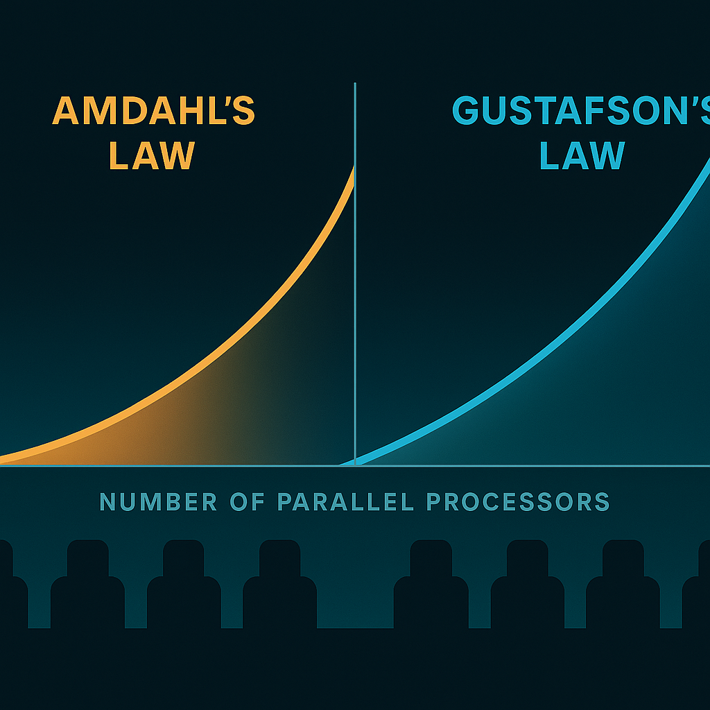
Amdahl’s Law and Gustafson’s Law are often presented as opposites, but they model different scenarios.
- Amdahl assumes a fixed problem size and asks: how much faster can I make this workload with P processors when a fraction s is inherently serial? The upper bound is:
$$\text{Speedup}_A(P) = \frac{1}{s + \frac{1-s}{P}}.$$
- Gustafson assumes a fixed execution time and asks: given P processors, how much bigger can the problem become if parallel parts scale? The scaled speedup is:
$$\text{Speedup}_G(P) = s + (1-s),P.$$
Neither law is “wrong.” Use Amdahl when the dataset is fixed (e.g., an SLA-bound query), and Gustafson when capacity grows with resources (e.g., larger simulations).
Practical considerations
- The “serial fraction” s is not constant. It changes with cache behavior, synchronization, I/O, and algorithmic choices.
- Contention and communication impose additional overhead. On NUMA machines and clusters, the effective 1/P region often degrades to 1/(P^α) for some α < 1 due to bandwidth and latency.
- Weak vs. strong scaling tests quantify these effects. Run both.
A quick experiment sketch
If you have a parallel kernel K and a serial setup S, measure wall times for varying P:
- Strong scaling: hold input size fixed; plot T(P). Compare empirical speedup with Amdahl.
- Weak scaling: grow input size with P; check if time stays flat. Compare with Gustafson expectations.
The punchline: choose your model based on product constraints (fixed time or fixed size), and validate with real measurements.
1. Historical Context & Motivation
Gene Amdahl introduced his law in 1967 to inject realism into expectations around adding processors to a system that runs a fixed workload (e.g., a benchmark problem size defined by an institution or an SLA‑bounded transaction). Later, John Gustafson (late 1980s) observed that in many scientific and data‑driven domains, problem sizes expand to absorb available compute time: researchers scale resolution, dimensionality, iteration counts, or ensemble size. Thus, holding execution time roughly constant while scaling problem size changes the algebra of perceived speedup. The supposed “contradiction” is simply that they answer different questions:
| Question | Constraint | Varies | Appropriate Law |
|---|---|---|---|
| “If I add cores, how much faster does this fixed job finish?” | Problem size fixed | Time | Amdahl |
| “If I add cores but keep wall time the same, how much bigger a job can I run?” | Time budget fixed | Problem size | Gustafson |
2. Formal Derivations & Intuition
Amdahl (Strong Scaling)
Let a fraction ( s ) of execution be inherently serial and ( (1-s) ) be perfectly parallelizable. With ( P ) processors, the parallel portion ideally takes ( (1-s)/P ) of the original time, so normalized runtime is: $$ T’(P) = s + \frac{1-s}{P}. $$ Speedup is original time over new time: $$ SA(P) = \frac{1}{s + \frac{1-s}{P}}. $$ As ( P \to \infty ), ( S_A(P) \to 1/s ). Thus, _diminishing returns appear once ( P \gg (1-s)/s ).
Gustafson (Weak / Scaled Scaling)
Assume we scale the parallel part proportionally to ( P ) while keeping wall time ~1. Let the original serial work still consume fraction ( s ) of the new runtime. Total scaled work executed relative to the single‑processor baseline is: $$ W(P) = s + (1-s)P. $$ Interpreting this as an effective speedup vs. the single‑processor doing the same enlarged workload gives Gustafson’s form: $$ S_G(P) = s + (1-s)P. $$ Here, the linear term dominates for large ( P ) unless ( s ) grows.
Reconciling Them
If the serial fraction itself shrinks with larger problems (e.g., I/O or setup overhead amortizes), Gustafson’s optimistic scaling can still be bounded by other overheads (memory bandwidth, network contention) not in the simple algebra. In practice real speedup curves usually lie between naïve linear and Amdahl’s pessimistic upper bound.
3. Decomposing the “Serial Fraction”
The parameter ( s ) often bundles multiple phenomena:
- Truly sequential algorithmic stages (e.g., a final aggregation requiring ordered traversal).
- Critical sections or locks (mutual exclusion reducing effective parallelism).
- Communication & synchronization overhead (barriers, reductions, broadcast latency).
- Load imbalance causing some workers to idle.
- Resource contention (memory controllers, caches, interconnect bandwidth) flattening throughput.
We can refine Amdahl’s model: $$ T’(P) = s*{alg} + s*{sync}(P) + s*{imb}(P) + \frac{1-s*{alg}}{P*{eff}(P)} $$ Where ( P*{eff}(P) \le P ) incorporates loss due to contention. Measuring / estimating each component directs optimization effort.
4. Numerical Examples
Assume baseline runtime 100 seconds, with measured breakdown: 10 s serial init, 85 s parallel region, 5 s reduction. The “serial” parts sum to 15% (( s=0.15 )). Predicted Amdahl speedups:
| P | Speedup S_A | Time (s) |
|---|---|---|
| 1 | 1.00 | 100.0 |
| 2 | 1.74 | 57.5 |
| 4 | 2.70 | 37.0 |
| 8 | 3.64 | 27.5 |
| 16 | 4.32 | 23.1 |
| 32 | 4.71 | 21.2 |
| 64 | 4.90 | 20.4 |
Notice doubling cores past 16 yields small benefits. If we optimize the reduction (5 s) down to 1 s (now serial = 11/100 = 0.11): theoretical max jumps to ~9.09 vs. previous 6.67. Reducing serial work often beats adding hardware.
Under weak scaling, if we hold time near 100 s but enlarge the parallel portion linearly with ( P ), the executed useful work measured against the baseline is ( S_G(P) ). With ( s=0.15 ): at 32 cores, ( S_G=0.15 + 0.85*32 = 27.35 ) “effective” speedup in problem size.
5. Memory Hierarchy & Bandwidth Effects
Even if code is “parallel,” memory bandwidth can cap speedup. Suppose per‑core memory demand drives total bandwidth past system limits; effective per-core throughput scales sublinearly. We can model that as: $$ P*{eff}(P) = \min\left(P, \frac{B*{max}}{b_{core}}\right). $$ If each core wants 5 GB/s and the socket sustains 200 GB/s, linear scaling stops past 40 cores even if algorithmic parallelism remains. This interacts with both laws—Amdahl’s serial fraction effectively grows because the “parallel” region inflates in time relative to ideal.
6. Multi-Level Parallelism
Modern systems layer parallelism: vector (SIMD) lanes, cores, NUMA domains, nodes, GPUs, and possibly accelerators (TPUs). The composite speedup is multiplicative only if inefficiencies are independent. Practically, you evaluate scaling at each tier:
- Vectorization (SSE/AVX/GPU warps).
- Thread (OpenMP / pthreads) across cores.
- Process / rank (MPI) across nodes.
- Task / pipeline parallelism (asynchronous I/O, overlapping compute & comms).
Often a small serial fraction at one layer becomes dominant after you eliminate bottlenecks elsewhere. Continuous profiling (e.g., using Linux perf, VTune, Nsight Systems) is essential.
7. Overheads Hidden in Gustafson’s Framing
Gustafson’s expression omits that expanding problem size may increase the serial fraction: initialization of larger grids, building bigger data structures, or longer reduction trees. Empirically, ( s ) can be modeled as ( s(P) = s_0 + c \log P ) (e.g., tree reductions). Plugging this into scaled speedup: $$ S_G’(P) = s(P) + (1-s(P))P $$ reveals eventual deviation from linearity.
8. Measurement Methodology
Steps to obtain credible scaling curves:
- Baseline profiling: measure wall time, break down by phase; identify candidate serial components.
- Instrument barriers & reductions: timestamp entry/exit to quantify synchronization cost.
- Vary P systematically: run powers of two; collect (runtime, energy if relevant). Repeat for statistical confidence (variance can hide inflection points).
- Compute efficiency: ( E(P)=S(P)/P ). Watch where efficiency drops below thresholds (e.g., 50%).
- Fit models: simple regression to estimate ( s ); compare predicted vs observed; residual structure hints at unmodeled overhead.
- Iterate optimization: attack largest residual contributor; re-measure.
9. Extensions: Karp–Flatt Metric
The Karp–Flatt serial fraction estimate: $$ e(P) = \frac{1/S(P) - 1/P}{1 - 1/P} $$ provides an observed effective serial fraction including all overheads. Plotting ( e(P) ) vs. ( P ) reveals trends: if it grows, you are encountering scaling penalties (communication, imbalance). Amdahl’s “s” is constant only in ideal cases.
10. Accelerators (GPUs) & Heterogeneous Speedup
Porting a parallel region to a GPU changes relative weights. Suppose compute kernel becomes 20× faster but data marshaling (CPU↔GPU transfers, kernel launch) adds a fixed overhead. New serial fraction might increase if transfers dominate at small problem sizes, reducing strong scaling benefit until you scale problem size (Gustafson scenario) to amortize overhead.
Simple Model
Let original time = 1; parallel portion = 0.8 moved to GPU with speedup 20; transfer+launch overhead = 0.05 added to serial fraction. New time: $$ T’ = (0.2 + 0.05) + \frac{0.8}{20} = 0.25 + 0.04 = 0.29 $$ Speedup ≈ 3.45× not 20×. Optimizing data movement (overlapping transfers, using pinned memory, kernel fusion) reduces the additive overhead making the GPU scale more like its theoretical compute advantage.
11. Diminishing Returns & Cost Models
Hardware cost and energy scale roughly with ( P ). If speedup saturates, cost per unit work improves only up to the “knee” of the curve. Introduce a cost function: $$ \text{Cost Efficiency}(P)=\frac{S(P)}{P^\beta} $$ with ( \beta\approx1 ) (linear cost). Choose ( P ) maximizing this. Real deployments often target energy to solution: measure joules using RAPL or GPU telemetry; energy often bottoms near the same region where parallel efficiency degrades.
12. Common Misinterpretations
| Myth | Clarification |
|---|---|
| “Amdahl says adding more than N cores is pointless.” | No: it bounds speedup for that fixed problem. Bigger problems can still benefit. |
| “Gustafson guarantees linear scaling.” | Only if serial fraction stays constant and parallel work increases ideally. |
| “Serial fraction is inherent to language/runtime.” | Much is algorithm + data structure choice + synchronization strategy. |
| “Observed efficiency drop means algorithm is bad.” | Could be memory bandwidth saturation or network contention, not algorithmic serialism. |
13. Practical Checklist
- Define scaling objective: reduce time to answer (Amdahl) or increase resolution (Gustafson).
- Profile to partition time; quantify synchronization & imbalance.
- Fit early data to Amdahl; estimate potential upper bound—do not over‑invest beyond it.
- Evaluate memory / I/O throughput counters to find bandwidth ceilings.
- Explore algorithmic changes (e.g., more parallel-friendly data layouts) before hardware scaling.
- For weak scaling, track how serial initialization grows—keep it sublinear.
- Revisit at new hardware generations; architectural shifts (cache sizes, NUMA topology) change effective ( s ).
14. Tooling & Instrumentation Tips
- Use
perf stat -d(Linux) or VTune to examine instructions per cycle (IPC) shifts as P grows. - Insert high-resolution timers (TSC, chrono) around barriers to compute aggregate lost time.
- Use tracing (e.g., OpenTelemetry spans for distributed tasks) to isolate stragglers.
- For GPU: Nsight Systems to overlap copy/compute; Nsight Compute for memory transactions; watch achieved occupancy vs. theoretical.
- For MPI:
mpiPor built-in profiling interface to aggregate time in collectives.
15. Putting It Together: Mini Case Study
A simulation code (baseline 1 hour on 1 core): 8% serial setup, 90% parallel kernel, 2% I/O flush. On 32 cores measured speedup is only 10× (instead of ~11.6 predicted by Amdahl with s=0.08). Investigation shows cache misses doubling due to data structure layout. After restructuring arrays-of-structs to struct-of-arrays, kernel memory bandwidth improves; speedup rises to 11.2×. Further improvement stalls—profiling reveals barrier imbalance (some threads idle). Applying domain decomposition with better partitioning trims imbalance; final speedup 11.5×, near theoretical. Decision: scaling beyond 32 cores offers <5% gain; resources invested in increasing problem resolution instead (Gustafson scenario).
16. Further Reading (Titles)
- “The Validity of Amdahl’s Law in the Multicore Era” (analysis papers)
- “A Case for Optimistic Parallelism” (explores overhead and contention)
- “Roofline: An Insightful Visual Performance Model” (memory vs compute bounds)
- “The Karp–Flatt Metric for Parallel Performance” (derivation discussions)
- “Gustafson’s Scaling Revisited” (weak scaling nuances)
- Vendor profiling guides (Intel VTune, NVIDIA Nsight) for practical measurement.
17. Summary
Amdahl’s Law bounds speedup for fixed workloads by highlighting that serial portions dominate with many processors. Gustafson’s Law reframes scaling for expanding workloads under fixed time budgets. Real systems interpose memory bandwidth, synchronization, and imbalance, making effective scaling a function of more than an algorithmic serial fraction. Use both perspectives: Amdahl to judge when to stop adding cores, Gustafson to decide how to spend newly available cores. Always ground assumptions in measurement.