B-Trees and LSM-Trees: The Foundations of Modern Storage Engines

2021-07-14 · Leonardo Benicio

An in-depth exploration of B-Trees and LSM-Trees, the two dominant data structures powering databases from PostgreSQL to RocksDB. Learn their trade-offs, internal mechanics, and when to choose each for your workload.

Every database faces the same fundamental challenge: how do you organize data on disk so that both reads and writes are fast? Two data structures have emerged as the dominant answers—B-Trees and LSM-Trees. Understanding their trade-offs is essential for anyone building or operating data-d31dd26 systems. This post explores both in depth, from their internal mechanics to their real-world implementations.

1. The Storage Engine Problem

Before diving into specific data structures, let’s understand what we’re optimizing for.

1.1 The Read-Write Trade-off

Disk storage has fundamentally different characteristics than memory:

Sequential access is fast: Reading or writing data in order is 100-1000x faster than random access on HDDs, and still 10x faster on SSDs
Random access is slow: Seeking to arbitrary locations has high latency
Writes are especially expensive: SSDs wear out with writes, and HDDs have mechanical seek overhead

This creates a fundamental tension:

Optimize for reads: Keep data sorted and organized for fast lookups
Optimize for writes: Append data sequentially to avoid random I/O

No data structure can be optimal for both. B-Trees and LSM-Trees represent different points on this trade-off spectrum.

1.2 Key Operations

Storage engines must support these operations efficiently:

class StorageEngine:
    def put(self, key: bytes, value: bytes) -> None:
        """Insert or update a key-value pair."""
        pass
    
    def get(self, key: bytes) -> Optional[bytes]:
        """Retrieve the value for a key, or None if not found."""
        pass
    
    def delete(self, key: bytes) -> None:
        """Remove a key-value pair."""
        pass
    
    def scan(self, start_key: bytes, end_key: bytes) -> Iterator[Tuple[bytes, bytes]]:
        """Iterate over all key-value pairs in a range."""
        pass

The relative frequency of these operations determines which data structure is optimal.

1.3 Metrics That Matter

When evaluating storage engines:

Write amplification: How many times is data written to disk for each logical write?
Read amplification: How many disk reads are needed for each logical read?
Space amplification: How much extra disk space is used beyond the logical data size?
Latency distribution: Not just averages, but P99 and P999 latencies

B-Trees and LSM-Trees make different trade-offs across these metrics.

2. B-Trees: The Read-Optimized Classic

B-Trees have powered relational databases for over 50 years. They’re the default choice for PostgreSQL, MySQL InnoDB, SQL Server, and Oracle.

2.1 Structure and Invariants

A B-Tree is a self-balancing tree where:

Each node contains multiple keys in sorted order
Internal nodes contain pointers to child nodes
All leaves are at the same depth
Nodes are sized to match disk pages (typically 4KB-16KB)

                    [30 | 60]
                   /    |    \
                  /     |     \
          [10|20]    [40|50]   [70|80|90]
          /  |  \    /  |  \    /  |  |  \
        [...] [...] [...] [...] [...] [...]

Key invariants for a B-Tree of order m:

Each node has at most m children
Each node (except root) has at least ⌈m/2⌉ children
The root has at least 2 children (if not a leaf)
All leaves appear at the same level

2.2 B+ Trees: The Practical Variant

Most databases use B+ Trees, which differ from B-Trees:

Only leaves contain values: Internal nodes contain only keys and pointers
Leaves are linked: A doubly-linked list connects all leaves for efficient range scans
Higher fanout: More keys per internal node means shallower trees

Internal nodes (keys only):
                    [30 | 60]
                   /    |    \
          [10|20]    [40|50]   [70|80|90]

Leaf nodes (keys + values, linked):
[10:v1|20:v2] <-> [30:v3|40:v4|50:v5] <-> [60:v6|70:v7|80:v8|90:v9]

2.3 Point Lookup

Finding a key in a B+ Tree:

def get(self, key):
    node = self.root
    
    while not node.is_leaf:
        # Binary search within the node
        i = binary_search(node.keys, key)
        node = node.children[i]
    
    # Binary search in leaf
    i = binary_search(node.keys, key)
    if i < len(node.keys) and node.keys[i] == key:
        return node.values[i]
    return None

With pages sized to match disk blocks, each level requires one disk read. A B+ Tree with 1000 keys per node and 1 billion entries needs only 3 levels—just 3 disk reads for any lookup.

2.4 Insertion

Inserting a key-value pair:

def put(self, key, value):
    # Find the leaf where this key belongs
    leaf, path = self.find_leaf_with_path(key)
    
    # Insert into leaf
    leaf.insert(key, value)
    
    # If leaf is too full, split
    if leaf.is_overfull():
        self.split_and_propagate(leaf, path)

def split_and_propagate(self, node, path):
    # Split the node in half
    mid = len(node.keys) // 2
    left_node = node.keys[:mid]
    right_node = node.keys[mid:]
    middle_key = node.keys[mid]
    
    # Propagate split to parent
    if path:
        parent = path.pop()
        parent.insert_child(middle_key, right_node)
        
        if parent.is_overfull():
            self.split_and_propagate(parent, path)
    else:
        # Split the root - tree grows taller
        new_root = Node([middle_key], [left_node, right_node])
        self.root = new_root

Splits cascade upward, potentially all the way to the root. The tree grows from the bottom up, maintaining balance.

2.5 Deletion

Deletion is more complex because nodes might become underfull:

def delete(self, key):
    leaf, path = self.find_leaf_with_path(key)
    leaf.remove(key)
    
    if leaf.is_underfull() and path:
        self.rebalance(leaf, path)

def rebalance(self, node, path):
    parent = path[-1]
    sibling = self.get_sibling(node, parent)
    
    if sibling.can_lend():
        # Borrow from sibling
        self.redistribute(node, sibling, parent)
    else:
        # Merge with sibling
        merged = self.merge(node, sibling)
        parent.remove_child(node)
        
        if parent.is_underfull() and len(path) > 1:
            self.rebalance(parent, path[:-1])

2.6 Concurrency Control

B-Trees require careful locking for concurrent access:

Latch crabbing: Hold a latch on the parent while acquiring the child’s latch, then release the parent:

def get_concurrent(self, key):
    node = self.root
    node.acquire_read_latch()
    
    while not node.is_leaf:
        child_idx = binary_search(node.keys, key)
        child = node.children[child_idx]
        
        child.acquire_read_latch()
        node.release_read_latch()  # Safe to release parent
        node = child
    
    result = node.get(key)
    node.release_read_latch()
    return result

Optimistic locking: For writes, optimistically assume no splits will cascade to the root:

def put_optimistic(self, key, value):
    # First, try optimistic path (no root latch)
    leaf, path = self.find_leaf_with_latches(key, write_latch=True)
    
    leaf.insert(key, value)
    
    if leaf.is_overfull():
        if self.can_handle_locally(leaf, path):
            self.split_and_propagate(leaf, path)
        else:
            # Restart with pessimistic locking from root
            self.release_all_latches(path)
            self.put_pessimistic(key, value)
    
    self.release_all_latches(path)

2.7 Write-Ahead Logging

B-Tree modifications must be crash-safe. Write-ahead logging (WAL) ensures durability:

def put_with_wal(self, key, value):
    # 1. Write to WAL first
    log_record = LogRecord(
        type="INSERT",
        key=key,
        value=value,
        page_id=target_page.id,
        old_value=target_page.get(key)
    )
    self.wal.append(log_record)
    self.wal.flush()  # Ensure on disk
    
    # 2. Modify the page in memory
    target_page.insert(key, value)
    
    # 3. Eventually write dirty pages to disk (checkpoint)
    # Pages can be written in any order - WAL ensures recoverability

3. LSM-Trees: The Write-Optimized Alternative

Log-Structured Merge-Trees (LSM-Trees) were designed for write-heavy workloads. They power RocksDB, LevelDB, Cassandra, HBase, and many modern databases.

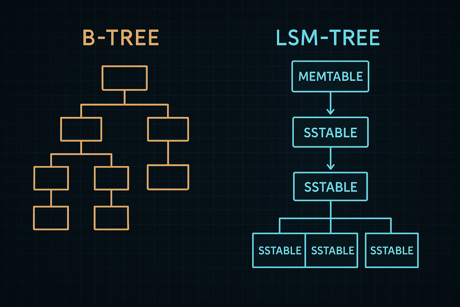
3.1 Core Idea

Instead of modifying data in place, LSM-Trees:

Buffer writes in memory (memtable)
Flush full memtables to disk as immutable sorted files (SSTables)
Periodically merge SSTables in the background (compaction)

Writes → [Memtable] → Flush → [L0 SSTables] → Compact → [L1] → ... → [Ln]

Memory:
┌─────────────────┐
│   Memtable      │  ← All writes go here first
│ (sorted, mutable)│
└─────────────────┘

Disk:
┌─────────────────┐
│   Level 0       │  ← Recently flushed, may overlap
│ SST SST SST     │
├─────────────────┤
│   Level 1       │  ← Compacted, non-overlapping
│ SST SST SST SST │
├─────────────────┤
│   Level 2       │  ← Larger, non-overlapping
│ SST SST SST ... │
└─────────────────┘

3.2 The Memtable

The memtable is an in-memory sorted data structure—typically a skip list or red-black tree:

class Memtable:
    def __init__(self, max_size):
        self.data = SkipList()  # Or RedBlackTree
        self.size = 0
        self.max_size = max_size
        self.wal = WriteAheadLog()
    
    def put(self, key, value):
        # Write to WAL for durability
        self.wal.append(key, value)
        
        # Insert into sorted structure
        self.data.insert(key, value)
        self.size += len(key) + len(value)
    
    def get(self, key):
        return self.data.get(key)
    
    def is_full(self):
        return self.size >= self.max_size
    
    def flush_to_sstable(self, path):
        # Write sorted data to disk
        with SSTableWriter(path) as writer:
            for key, value in self.data.iterate():
                writer.write(key, value)
        
        # Clear WAL after successful flush
        self.wal.truncate()

3.3 SSTables (Sorted String Tables)

SSTables are immutable files containing sorted key-value pairs:

SSTable File Structure:
┌─────────────────────────────────────────┐
│ Data Block 1                            │
│   key1:value1, key2:value2, ...         │
├─────────────────────────────────────────┤
│ Data Block 2                            │
│   key100:value100, key101:value101, ... │
├─────────────────────────────────────────┤
│ ...                                     │
├─────────────────────────────────────────┤
│ Index Block                             │
│   block1_last_key → offset              │
│   block2_last_key → offset              │
├─────────────────────────────────────────┤
│ Bloom Filter                            │
│   (probabilistic membership test)       │
├─────────────────────────────────────────┤
│ Footer (metadata)                       │
└─────────────────────────────────────────┘

Key features:

Block-based: Data is organized into fixed-size blocks for efficient I/O
Sparse index: Only boundary keys are indexed, not every key
Bloom filter: Quickly determine if a key might exist (avoiding disk reads)
Compression: Blocks are typically compressed (LZ4, Snappy, Zstd)

3.4 Point Lookup

Reading from an LSM-Tree requires checking multiple levels:

class LSMTree:
    def get(self, key):
        # 1. Check memtable first (most recent data)
        value = self.memtable.get(key)
        if value is not None:
            return None if value == TOMBSTONE else value
        
        # 2. Check immutable memtables (being flushed)
        for imm in reversed(self.immutable_memtables):
            value = imm.get(key)
            if value is not None:
                return None if value == TOMBSTONE else value
        
        # 3. Check SSTables from newest to oldest
        for level in self.levels:
            for sstable in level.get_candidates(key):
                # Check bloom filter first
                if not sstable.bloom_filter.might_contain(key):
                    continue
                
                value = sstable.get(key)
                if value is not None:
                    return None if value == TOMBSTONE else value
        
        return None

This is the read amplification problem: a single lookup might check many SSTables.

3.5 Compaction

Compaction merges SSTables to reduce read amplification and reclaim space:

def compact_level(self, level):
    """Merge SSTables from level L into level L+1."""
    # Select SSTables to compact
    input_sstables = self.select_for_compaction(level)
    
    # Find overlapping SSTables in next level
    key_range = self.get_key_range(input_sstables)
    target_sstables = self.levels[level + 1].get_overlapping(key_range)
    
    # Merge-sort all inputs
    merged = MergingIterator(input_sstables + target_sstables)
    
    # Write new SSTables
    new_sstables = []
    writer = SSTableWriter()
    
    for key, value in merged:
        # Skip older versions of the same key
        if key == last_key:
            continue
        
        # Skip tombstones at the bottom level
        if value == TOMBSTONE and level + 1 == self.max_level:
            continue
        
        writer.write(key, value)
        
        if writer.size >= self.target_sstable_size:
            new_sstables.append(writer.finish())
            writer = SSTableWriter()
    
    # Atomically swap old SSTables for new ones
    self.apply_compaction(
        level=level,
        old_sstables=input_sstables + target_sstables,
        new_sstables=new_sstables
    )

3.6 Compaction Strategies

Different strategies trade off write amplification, space amplification, and read performance:

Leveled Compaction (LevelDB, RocksDB default):

Each level is 10x larger than the previous
Non-overlapping SSTables within each level (except L0)
Low space amplification (~1.1x)
Higher write amplification (10-30x)

L0: [SST] [SST] [SST]     ← Overlapping, recently flushed
L1: [--|--|--]            ← 10MB total, non-overlapping
L2: [--|--|--|--|--|--]   ← 100MB total, non-overlapping
L3: [--|--|--|--|--|...] ← 1GB total, non-overlapping

Size-Tiered Compaction (Cassandra, HBase):

Group SSTables by size
Merge SSTables of similar size together
Lower write amplification (4-8x)
Higher space amplification (up to 2x)

Tier 1: [small] [small] [small] [small] → merge → [medium]
Tier 2: [medium] [medium] [medium]      → merge → [large]
Tier 3: [large] [large]                 → merge → [huge]

FIFO Compaction:

Simply delete oldest SSTables
Useful for time-series data with TTL

Universal Compaction (RocksDB):

Hybrid approach balancing write and space amplification
Adapts based on workload characteristics

3.7 Bloom Filters

Bloom filters dramatically reduce read amplification:

class BloomFilter:
    def __init__(self, expected_items, false_positive_rate=0.01):
        # Calculate optimal size and hash count
        self.size = self.optimal_size(expected_items, false_positive_rate)
        self.num_hashes = self.optimal_hashes(self.size, expected_items)
        self.bits = bitarray(self.size)
    
    def add(self, key):
        for i in range(self.num_hashes):
            idx = self.hash(key, i) % self.size
            self.bits[idx] = 1
    
    def might_contain(self, key):
        for i in range(self.num_hashes):
            idx = self.hash(key, i) % self.size
            if not self.bits[idx]:
                return False  # Definitely not present
        return True  # Might be present (possible false positive)

With a 1% false positive rate, a bloom filter uses about 10 bits per key. For an SSTable with 1 million keys, the bloom filter is only ~1.2MB—easily cached in memory.

3.8 Deletions and Tombstones

LSM-Trees handle deletions with tombstones—special markers indicating a key is deleted:

def delete(self, key):
    # Write a tombstone marker
    self.put(key, TOMBSTONE)

Tombstones are removed during compaction at the bottom level:

def should_keep_during_compaction(self, key, value, level):
    if value != TOMBSTONE:
        return True
    
    # Keep tombstones until they reach the bottom level
    # (to shadow older versions in lower levels)
    if level < self.max_level:
        return True
    
    # At bottom level, tombstone can be removed
    return False

This means deleted data isn’t immediately reclaimed—space is freed only after compaction propagates tombstones to the bottom.

4. B-Trees vs. LSM-Trees: The Trade-offs

4.1 Write Performance

LSM-Trees win for writes:

Sequential I/O for all writes (memtable flush, compaction)
Batching amortizes overhead
Write amplification: 10-30x (leveled) or 4-8x (size-tiered)

B-Trees have higher write cost:

Random I/O for in-place updates
Each write modifies a specific page
Write amplification: ~2x (page + WAL)

However, B-Trees have lower tail latency—no background compaction causing jitter.

4.2 Read Performance

B-Trees win for point reads:

Guaranteed O(log n) with ~3-4 disk reads for billion-key datasets
No need to check multiple files
Consistent, predictable latency

LSM-Trees have higher read cost:

Must check multiple levels
Bloom filters help but aren’t perfect
Read amplification can be 10x+ without careful tuning

4.3 Space Efficiency

LSM-Trees can be more efficient:

Compression is more effective on sorted, immutable blocks
No page fragmentation
But tombstones and multiple versions consume space temporarily

B-Trees have consistent space usage:

Pages can be partially filled (typically 70-80%)
No temporary space overhead from compaction
Fragmentation over time requires rebuilding

4.4 Summary Table

Metric	B-Tree	LSM-Tree
Write throughput	Lower	Higher
Write latency	Consistent	Variable (compaction)
Point read	Faster	Slower
Range scan	Fast	Fast
Write amplification	~2x	10-30x
Read amplification	1x	1-10x
Space amplification	1.3-1.5x	1.1-2x
Concurrency	Complex	Simpler

5. Advanced B-Tree Techniques

5.1 Prefix Compression

Many keys share common prefixes. Compress them:

Without compression:
  "user:alice:profile"
  "user:alice:settings"
  "user:bob:profile"

With prefix compression:
  "user:alice:profile"
  [8]"settings"        ← Share 8 bytes with previous key
  [5]"bob:profile"     ← Share 5 bytes with previous key

This can reduce index size by 50% or more for certain key patterns.

5.2 Suffix Truncation

Internal nodes only need enough of the key to distinguish children:

Full keys in leaves:
  "application_server_1"
  "application_server_2"

Truncated separator in internal node:
  "application_server_1" vs "application_server_2"
  Can use just "application_server_2" as separator
  Or even just "2" if context is clear

5.3 Bulk Loading

Building a B-Tree from sorted data is much faster than individual inserts:

def bulk_load(sorted_data, page_size):
    """Build a B-Tree from sorted data, bottom-up."""
    # Create leaf pages
    leaves = []
    current_page = Page()
    
    for key, value in sorted_data:
        if current_page.is_full():
            leaves.append(current_page)
            current_page = Page()
        current_page.add(key, value)
    
    if not current_page.is_empty():
        leaves.append(current_page)
    
    # Link leaves
    for i in range(len(leaves) - 1):
        leaves[i].next = leaves[i + 1]
    
    # Build internal nodes bottom-up
    current_level = leaves
    while len(current_level) > 1:
        next_level = []
        current_page = InternalPage()
        
        for page in current_level:
            if current_page.is_full():
                next_level.append(current_page)
                current_page = InternalPage()
            current_page.add_child(page.first_key(), page)
        
        if not current_page.is_empty():
            next_level.append(current_page)
        
        current_level = next_level
    
    return BTree(root=current_level[0])

Bulk loading achieves 100% page fill factor and optimal layout.

5.4 Copy-on-Write B-Trees

Instead of in-place updates, create new pages:

def put_cow(self, key, value):
    """Copy-on-write insertion."""
    path = self.find_path(key)
    
    # Create new leaf with the update
    new_leaf = path[-1].copy()
    new_leaf.insert(key, value)
    
    # Propagate new pages up to root
    for i in range(len(path) - 2, -1, -1):
        new_node = path[i].copy()
        new_node.replace_child(path[i + 1], new_pages[-1])
        new_pages.append(new_node)
    
    # Atomic root pointer swap
    self.root = new_pages[-1]
    
    # Old pages can be garbage collected

Benefits:

Crash safety: No torn writes (old tree is always consistent)
Snapshots: Keep old root for point-in-time reads
Concurrency: Readers never block writers

Used by LMDB, BoltDB, and some file systems (Btrfs, ZFS).

6. Advanced LSM-Tree Techniques

6.1 Partitioned Indexes

Instead of one global index, partition by key range:

class PartitionedLSM:
    def __init__(self, num_partitions):
        self.partitions = [LSMTree() for _ in range(num_partitions)]
    
    def get_partition(self, key):
        # Consistent hashing or range-based partitioning
        return self.partitions[hash(key) % len(self.partitions)]
    
    def put(self, key, value):
        self.get_partition(key).put(key, value)
    
    def get(self, key):
        return self.get_partition(key).get(key)

Benefits:

Parallel compaction across partitions
Better cache locality
Isolation of hot key ranges

6.2 Tiered + Leveled Hybrid

Combine size-tiered compaction at L0-L1 with leveled compaction below:

L0: [SST] [SST] [SST] [SST]  ← Size-tiered (fast ingestion)
L1: [SST] [SST] [SST]        ← Size-tiered (buffer)
L2: [--|--|--|--|--|--]      ← Leveled (good read performance)
L3: [--|--|--|--|--|...]     ← Leveled

This balances write throughput (size-tiered at top) with read performance (leveled at bottom).

6.3 Remote Compaction

Offload compaction to dedicated servers:

class RemoteCompaction:
    def compact(self, sstables):
        # Upload SSTables to compaction server
        uploaded = self.upload_to_remote(sstables)
        
        # Request compaction
        job_id = self.compaction_service.submit(uploaded)
        
        # Wait for result
        result = self.compaction_service.wait(job_id)
        
        # Download compacted SSTables
        return self.download_result(result)

Benefits:

Compaction doesn’t consume local CPU/IO
Better resource isolation
Scales compaction independently

Used by Neon (Postgres), TiDB, and cloud-native databases.

6.4 Learned Indexes

Replace bloom filters with machine learning models:

class LearnedBloomFilter:
    def __init__(self, keys):
        # Train a model to predict key membership
        self.model = train_classifier(keys)
        
        # Backup bloom filter for false negatives
        self.backup_bloom = BloomFilter(false_negative_keys)
    
    def might_contain(self, key):
        if self.model.predict(key) > 0.5:
            return True
        return self.backup_bloom.might_contain(key)

Learned filters can achieve the same false positive rate with less memory—up to 70% savings in some workloads.

7. Hybrid Approaches

7.1 Bw-Tree (Microsoft)

Combines B-Tree structure with log-structured updates:

Base B-Tree pages are immutable
Updates are appended as delta records
Deltas are periodically consolidated

Page 42:
┌─────────────────┐
│  Delta: DEL(k5) │ → ┌─────────────────┐
└─────────────────┘   │  Delta: PUT(k3) │ → ┌─────────────────┐
                      └─────────────────┘   │  Base Page      │
                                            │  k1, k2, k3, k5 │
                                            └─────────────────┘

Benefits:

No write-ahead log needed (deltas are the log)
Latch-free operation using CAS
Used by Microsoft SQL Server Hekaton

7.2 Bε-Trees

Bε-Trees (B-epsilon trees) are a middle ground:

Like B-Trees, but internal nodes have buffers
Writes accumulate in buffers and trickle down
Asymptotically optimal for both reads and writes

Internal node:
┌─────────────────────────────────┐
│ Keys: [30 | 60]                 │
│ Children: [ptr1 | ptr2 | ptr3] │
│ Buffer: [(k15, v15), (k45, v45), (k72, v72)] │
└─────────────────────────────────┘

When buffer fills, flush entries to appropriate children.

Used by TokuDB (Percona), BetrFS.

7.3 COLA (Cache-Oblivious Lookahead Array)

Achieves optimal write performance without knowing cache/memory hierarchy:

Array of arrays, each double the previous size
Fractional cascading for efficient searches
Automatic adaptation to any cache size

8. Choosing the Right Storage Engine

8.1 Workload Analysis

Ask these questions:

Read/write ratio: >80% reads? B-Tree. Write-heavy? LSM-Tree.
Key access patterns: Hot keys? Uniform? Time-ordered?
Latency requirements: Need consistent P99? B-Tree. Can tolerate jitter? LSM-Tree.
Data size: Fits in memory? Either works. Much larger? Consider compaction I/O.
Durability requirements: Synchronous writes? Both can do it, but with different trade-offs.

8.2 Decision Matrix

Workload	Recommended	Reason
OLTP (transactions)	B-Tree	Consistent latency, point queries
Time-series	LSM-Tree	Sequential writes, range scans
Analytics	Columnar (not covered)	Aggregations, compression
Key-value cache	LSM-Tree	High write throughput
Mixed	Depends	Profile your workload

8.3 Tuning Parameters

For B-Trees:

Page size: Match filesystem/storage block size
Fill factor: Trade insert performance for space efficiency
Checkpoint frequency: Balance durability vs. I/O

For LSM-Trees:

Memtable size: Larger = fewer flushes, more memory
Level size ratio: 10x is typical; lower = more levels, less write amplification
Compaction threads: More parallelism, more I/O contention
Bloom filter bits per key: 10 bits ≈ 1% false positive

9. Debugging and Monitoring

9.1 Key Metrics

B-Tree:

class BTreeMetrics:
    def report(self):
        return {
            "height": self.tree.height(),
            "total_pages": self.tree.page_count(),
            "fill_factor": self.tree.average_fill_factor(),
            "cache_hit_rate": self.buffer_pool.hit_rate(),
            "checkpoint_lag": self.wal.checkpoint_lag(),
            "page_splits_per_sec": self.split_counter.rate(),
        }

LSM-Tree:

class LSMMetrics:
    def report(self):
        return {
            "memtable_size": self.memtable.size,
            "levels": [len(level.sstables) for level in self.levels],
            "pending_compaction_bytes": self.compaction_queue.total_bytes(),
            "write_stall_duration": self.stall_counter.total_ms(),
            "bloom_filter_useful": self.bloom_useful / self.bloom_checks,
            "read_amplification": self.disk_reads / self.logical_reads,
        }

9.2 Common Problems

B-Tree issues:

Page splits cascading: Bulk loading sorted data causes worst-case splits
Lock contention: Hot pages become bottlenecks
Checkpoint storms: Large buffer pools take long to flush

LSM-Tree issues:

Write stalls: Compaction can’t keep up with writes
Space amplification spikes: During compaction, old and new SSTables coexist
Read amplification: Too many L0 files or missing bloom filters

10. Real-World Implementations

10.1 PostgreSQL (B-Tree)

PostgreSQL’s B-Tree implementation is a masterclass in production engineering:

-- Create a B-Tree index
CREATE INDEX idx_users_email ON users (email);

-- Examine index structure
SELECT * FROM bt_metap('idx_users_email');
-- Returns: magic, version, root, level, fastroot, fastlevel, ...

-- Page-level inspection
SELECT * FROM bt_page_stats('idx_users_email', 1);
-- Returns: blkno, type, live_items, dead_items, avg_item_size, ...

Key implementation details:

MVCC integration: Index entries point to heap tuples, visibility checked at read time
HOT updates: Heap-Only Tuples avoid index updates for non-indexed column changes
Deferred splits: Splits are logged and can be replayed during recovery
Right-link pointers: Allow lock-free traversal of siblings during splits

10.2 RocksDB (LSM-Tree)

RocksDB is Facebook’s production LSM-Tree, used by TiKV, CockroachDB, and many others:

// Basic RocksDB usage
rocksdb::DB* db;
rocksdb::Options options;
options.create_if_missing = true;
options.write_buffer_size = 64 * 1024 * 1024;  // 64MB memtable
options.max_write_buffer_number = 3;
options.level0_file_num_compaction_trigger = 4;

rocksdb::Status status = rocksdb::DB::Open(options, "/tmp/testdb", &db);

db->Put(rocksdb::WriteOptions(), "key1", "value1");
std::string value;
db->Get(rocksdb::ReadOptions(), "key1", &value);

Key features:

Column families: Multiple LSM-Trees sharing one WAL
Prefix bloom filters: Efficient prefix scans
Rate limiter: Control compaction I/O impact
Blob storage: Large values stored separately for efficiency
Transactions: Optimistic and pessimistic transaction support

10.3 WiredTiger (Hybrid)

MongoDB’s WiredTiger combines B-Tree structure with LSM-like techniques:

Lookaside table: Buffers updates to reduce page churn
Hazard pointers: Lock-free concurrent access
Page reconciliation: Converts in-memory pages to on-disk format
Checkpoint curse prevention: Evicts pages incrementally

# MongoDB WiredTiger statistics
db.serverStatus().wiredTiger.cache
# Returns: bytes currently in cache, tracked dirty bytes, pages read/written

10.4 LMDB (Copy-on-Write B-Tree)

Lightning Memory-Mapped Database uses memory-mapped files with CoW B-Trees:

MDB_env *env;
mdb_env_create(&env);
mdb_env_set_mapsize(env, 10485760);  // 10MB
mdb_env_open(env, "./testdb", 0, 0644);

MDB_txn *txn;
MDB_dbi dbi;
mdb_txn_begin(env, NULL, 0, &txn);
mdb_dbi_open(txn, NULL, 0, &dbi);

MDB_val key = {3, "foo"};
MDB_val value = {3, "bar"};
mdb_put(txn, dbi, &key, &value, 0);
mdb_txn_commit(txn);

Key benefits:

Zero-copy reads: Direct memory access, no serialization
Single-writer, multi-reader: Simple concurrency model
Crash-proof: CoW ensures consistent state at all times
Small footprint: Minimal runtime dependencies

11. Storage Engine Evolution

11.1 Historical Context

The evolution of storage engines reflects changing hardware and workloads:

1970s-1990s: B-Tree Dominance

Disk seeks were expensive (10ms)
Sequential bandwidth was limited
B-Trees minimized seeks with high fanout
ISAM, B-Tree variants in mainframe databases

2000s: Log-Structured Renaissance

SSDs changed the calculus (no seek penalty)
Write amplification became critical (SSD wear)
LSM-Trees enabled write-heavy workloads
BigTable, LevelDB pioneered practical LSM implementations

2010s: Hybrid and Specialized

Cloud storage added network latency considerations
Tiered storage (memory, SSD, HDD) required adaptation
Learned indexes emerged from ML research
Persistent memory (Intel Optane) blurred memory/storage boundary

2020s: Disaggregated and Cloud-Native

Compute and storage separation
Remote compaction offloading
Object storage as primary persistence
Serverless databases with pay-per-query

11.2 Emerging Trends

Persistent Memory (PMEM):

Traditional assumptions break down with byte-addressable persistent memory:

// Intel Optane PMEM access
void *pmem_addr = pmem_map_file("/pmem/db", size, ...);
pmem_memcpy_persist(pmem_addr + offset, data, len);
// Data is durable after memcpy returns!

New data structures emerge:

FAST&FAIR: B-Tree variant for PMEM
SLM-DB: Single-level merge for PMEM
FPTree: Fingerprint-based tree for hybrid DRAM/PMEM

GPU-Accelerated Storage:

GPUs can accelerate certain storage operations:

// GPU-accelerated binary search
__global__ void parallel_lookup(Key* keys, int n, Key target, int* result) {
    int tid="ib35e80" * blockDim.x + threadIdx.x;
    // Each thread searches a portion
    int left = tid * (n / NUM_THREADS);
    int right = (tid + 1) * (n / NUM_THREADS) - 1;
    // Binary search in assigned range
    ...
}

Programmable Storage (Computational Storage):

Push computation to storage devices:

# Computational storage pseudo-code
def query_on_device(ssd, predicate):
    # Filter runs on SSD controller, not host CPU
    return ssd.execute(
        operation="SCAN",
        filter=predicate,
        projection=["id", "name"]
    )
    # Only matching rows cross the PCIe bus

11.3 The Future of Storage Engines

Several trends will shape storage engines:

Automatic tuning: ML-based configuration optimization
Workload-adaptive structures: Data structures that morph based on access patterns
Cross-layer optimization: Co-designing storage engine, file system, and device firmware
Sustainable storage: Energy-aware algorithms as data centers face power constraints
Verified implementations: Formal verification to eliminate subtle bugs

12. Implementing a Minimal Storage Engine

Let’s build a simple LSM-Tree from scratch to solidify understanding:

import os
import json
import struct
from collections import OrderedDict
from typing import Optional, Iterator, Tuple

class Memtable:
    """In-memory sorted buffer using an ordered dictionary."""
    
    def __init__(self, max_size: int = 1024 * 1024):
        self.data = OrderedDict()
        self.size = 0
        self.max_size = max_size
    
    def put(self, key: str, value: str) -> None:
        old_size = len(self.data.get(key, "")) + len(key) if key in self.data else 0
        self.data[key] = value
        self.size += len(key) + len(value) - old_size
        # Keep sorted
        self.data = OrderedDict(sorted(self.data.items()))
    
    def get(self, key: str) -> Optional[str]:
        return self.data.get(key)
    
    def delete(self, key: str) -> None:
        self.put(key, "__TOMBSTONE__")
    
    def is_full(self) -> bool:
        return self.size >= self.max_size
    
    def items(self) -> Iterator[Tuple[str, str]]:
        return iter(self.data.items())


class SSTable:
    """Immutable sorted string table on disk."""
    
    def __init__(self, path: str):
        self.path = path
        self.index = {}  # Sparse index: first key of each block
        self._load_index()
    
    @classmethod
    def create(cls, path: str, items: Iterator[Tuple[str, str]]) -> 'SSTable':
        """Create a new SSTable from sorted key-value pairs."""
        with open(path, 'wb') as f:
            for key, value in items:
                # Simple format: key_len (4 bytes), key, value_len (4 bytes), value
                key_bytes = key.encode('utf-8')
                value_bytes = value.encode('utf-8')
                f.write(struct.pack('I', len(key_bytes)))
                f.write(key_bytes)
                f.write(struct.pack('I', len(value_bytes)))
                f.write(value_bytes)
        
        return cls(path)
    
    def _load_index(self) -> None:
        """Load sparse index for faster lookups."""
        if not os.path.exists(self.path):
            return
        
        with open(self.path, 'rb') as f:
            offset = 0
            while True:
                pos = f.tell()
                key_len_bytes = f.read(4)
                if not key_len_bytes:
                    break
                
                key_len = struct.unpack('I', key_len_bytes)[0]
                key = f.read(key_len).decode('utf-8')
                value_len = struct.unpack('I', f.read(4))[0]
                f.seek(value_len, 1)  # Skip value
                
                # Index every 100th key for sparse index
                if offset % 100 == 0:
                    self.index[key] = pos
                offset += 1
    
    def get(self, key: str) -> Optional[str]:
        """Look up a key in the SSTable."""
        # Find starting position using sparse index
        start_pos = 0
        for indexed_key, pos in self.index.items():
            if indexed_key <= key:
                start_pos = pos
            else:
                break
        
        with open(self.path, 'rb') as f:
            f.seek(start_pos)
            while True:
                key_len_bytes = f.read(4)
                if not key_len_bytes:
                    break
                
                key_len = struct.unpack('I', key_len_bytes)[0]
                current_key = f.read(key_len).decode('utf-8')
                value_len = struct.unpack('I', f.read(4))[0]
                value = f.read(value_len).decode('utf-8')
                
                if current_key == key:
                    return None if value == "__TOMBSTONE__" else value
                if current_key > key:
                    break  # Key not found (data is sorted)
        
        return None
    
    def items(self) -> Iterator[Tuple[str, str]]:
        """Iterate over all key-value pairs."""
        with open(self.path, 'rb') as f:
            while True:
                key_len_bytes = f.read(4)
                if not key_len_bytes:
                    break
                
                key_len = struct.unpack('I', key_len_bytes)[0]
                key = f.read(key_len).decode('utf-8')
                value_len = struct.unpack('I', f.read(4))[0]
                value = f.read(value_len).decode('utf-8')
                
                yield key, value


class SimpleLSM:
    """A minimal LSM-Tree implementation."""
    
    def __init__(self, directory: str, memtable_size: int = 1024 * 1024):
        self.directory = directory
        os.makedirs(directory, exist_ok=True)
        
        self.memtable = Memtable(memtable_size)
        self.sstables = []
        self._load_sstables()
    
    def _load_sstables(self) -> None:
        """Load existing SSTables from disk."""
        for filename in sorted(os.listdir(self.directory)):
            if filename.endswith('.sst'):
                path = os.path.join(self.directory, filename)
                self.sstables.append(SSTable(path))
    
    def put(self, key: str, value: str) -> None:
        """Insert or update a key-value pair."""
        self.memtable.put(key, value)
        
        if self.memtable.is_full():
            self._flush()
    
    def get(self, key: str) -> Optional[str]:
        """Retrieve the value for a key."""
        # Check memtable first (most recent)
        value = self.memtable.get(key)
        if value is not None:
            return None if value == "__TOMBSTONE__" else value
        
        # Check SSTables from newest to oldest
        for sstable in reversed(self.sstables):
            value = sstable.get(key)
            if value is not None:
                return value
        
        return None
    
    def delete(self, key: str) -> None:
        """Delete a key by writing a tombstone."""
        self.memtable.delete(key)
        
        if self.memtable.is_full():
            self._flush()
    
    def _flush(self) -> None:
        """Flush memtable to disk as an SSTable."""
        timestamp = len(self.sstables)
        path = os.path.join(self.directory, f"{timestamp:08d}.sst")
        
        sstable = SSTable.create(path, self.memtable.items())
        self.sstables.append(sstable)
        
        self.memtable = Memtable(self.memtable.max_size)
    
    def compact(self) -> None:
        """Merge all SSTables into one (simple full compaction)."""
        if len(self.sstables) <= 1:
            return
        
        # Merge all SSTables
        merged = {}
        for sstable in self.sstables:
            for key, value in sstable.items():
                merged[key] = value
        
        # Remove tombstones and sort
        items = sorted(
            ((k, v) for k, v in merged.items() if v != "__TOMBSTONE__"),
            key=lambda x: x[0]
        )
        
        # Write new SSTable
        new_path = os.path.join(self.directory, "compacted.sst")
        new_sstable = SSTable.create(new_path, iter(items))
        
        # Remove old SSTables
        for sstable in self.sstables:
            os.remove(sstable.path)
        
        # Rename compacted file
        final_path = os.path.join(self.directory, "00000000.sst")
        os.rename(new_path, final_path)
        
        self.sstables = [SSTable(final_path)]


# Usage example
if __name__ == "__main__":
    db = SimpleLSM("/tmp/simple_lsm", memtable_size=1024)
    
    # Write some data
    for i in range(1000):
        db.put(f"key{i:04d}", f"value{i}")
    
    # Read it back
    print(db.get("key0042"))  # value42
    
    # Delete a key
    db.delete("key0042")
    print(db.get("key0042"))  # None
    
    # Compact
    db.compact()

This implementation demonstrates the core concepts while being readable. Production systems add:

Write-ahead logging for durability
Bloom filters for faster negative lookups
Block-based storage with compression
Concurrent access support
Leveled compaction with size thresholds

13. Summary

B-Trees and LSM-Trees represent two fundamental approaches to the storage engine problem:

B-Trees:

Optimized for reads with O(log n) guaranteed
In-place updates with write-ahead logging
Consistent latency, complex concurrency
Best for read-heavy OLTP workloads

LSM-Trees:

Optimized for writes with sequential I/O
Immutable SSTables with background compaction
Higher write throughput, variable latency
Best for write-heavy and time-series workloads

Key insights:

There is no free lunch: Every optimization trades off something else
Measure your workload: Synthetic benchmarks lie; profile production traffic
Hybrid approaches exist: Bw-Tree, Bε-Trees, and others blend the best of both
Tuning matters: Default configurations rarely match your specific needs
The right choice can change: As your workload evolves, re-evaluate

Understanding these data structures is foundational for anyone working with databases. Whether you’re choosing a database, tuning performance, or building storage systems, this knowledge transforms how you think about data persistence.