Cache‑Friendly Data Layouts: AoS vs. SoA (and the Hybrid In‑Between)

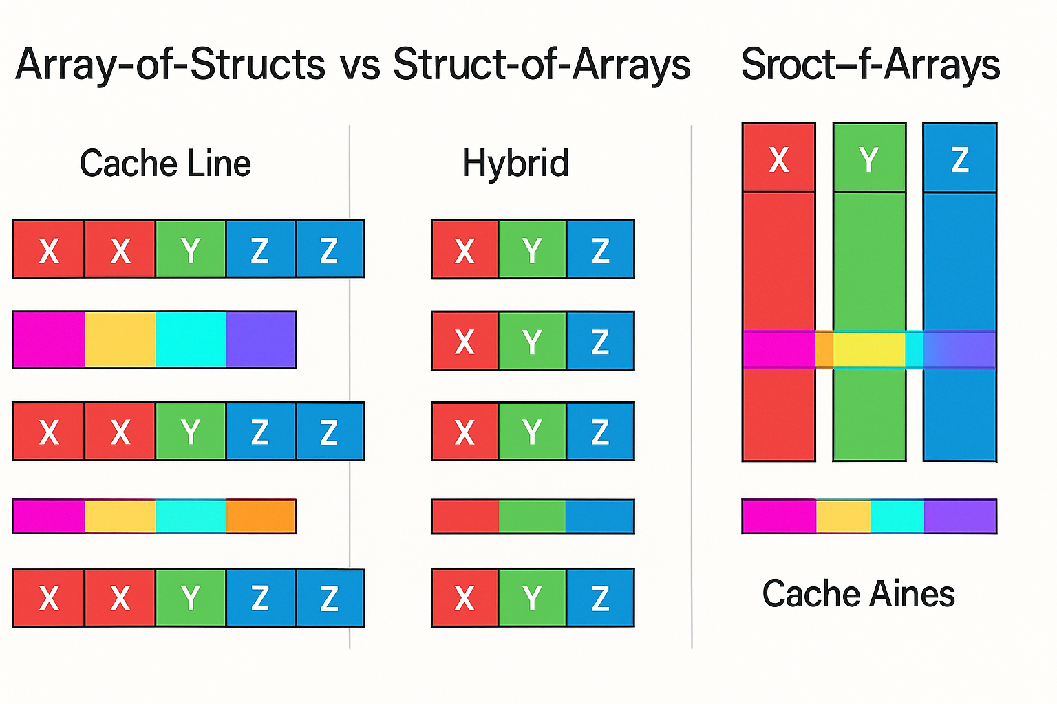
The fastest code you’ll ever write usually isn’t a brand‑new algorithm—it’s the same algorithm organized in memory so the CPU (or GPU) can consume it efficiently. That journey often starts with a deceptively small choice: Array‑of‑Structs (AoS) or Struct‑of‑Arrays (SoA). The layout you choose determines which cachelines move, which prefetchers trigger, how branch predictors behave, and whether SIMD units stay busy or starve.

In this post we’ll build an intuitive mental model for cachelines, TLBs, prefetchers, and vector units; examine AoS and SoA under realistic access patterns; then derive a hybrid (AoSoA) that quietly powers many high‑performance systems—from physics engines to databases to ML dataloaders. We’ll also walk through migration strategies, benchmarking pitfalls, and checklists you can apply this week.

The hardware model you actually need

You don’t need to memorize microarchitectural manuals to make good layout choices. A handful of truths carry most of the weight:

• Cachelines move in fixed‑size chunks (often 64 bytes on x86; 64–128 bytes on many ARM cores). Touch any byte, and the hardware drags the whole line. If your next access is within that line, it’s “free.” If not, you’ll pay again.
• Spatial locality feeds prefetchers. Sequential scans let the prefetcher stream upcoming lines; strided or data‑dependent jumps confuse it. SoA encourages contiguous scans through a single column.
• TLBs translate virtual to physical addresses. Many tiny pages blow your TLB; huge pages (2MB/1GB) reduce misses and page walks. Layout that encourages fewer, longer spans of memory tends to behave better.
• SIMD lanes like uniform, contiguous data. When values of the same field sit back‑to‑back (SoA), auto‑vectorization often “just works,” and intrinsics are trivial. With AoS, mixing fields across the line forces shuffles and scatter/gather.
• Branch predictors hate unpredictable control flow. If each entity takes a different branch, vector lanes idle. Grouping similar work (e.g., by field predicates) makes predictors and SIMD happier.

A final, underappreciated truth: bandwidth is cheap compared to latency when you’re already moving cachelines. If you’ll load a line anyway, packing the values you’ll actually use together can be more important than shrinking the total footprint.

AoS: Great for object‑wise work

Array‑of‑Structs keeps all fields of an entity together in memory. It shines when your per‑entity logic needs many fields and you traverse entities one by one. Game engines popularized AoS because “update this thing’s state” is a natural mental model.

Pros:

• Excellent locality for per‑object access: one line brings multiple fields you’ll touch immediately.
• Easy to reason about; fewer separate arrays to keep in sync; idiomatic in many languages.
• Friendly to heterogeneous branching per entity (each object can take a different path with limited overhead).

Cons:

• Wastes cache if you only need a subset of fields (dragging unused bytes on every access).
• Blocks wide SIMD on single columns; fields are interleaved, so vector lanes require gathers/shuffles.
• Padding and alignment can bloat memory; a couple of 64‑bit fields can explode line usage if you’re not careful.

A concrete AoS example

Suppose you maintain an array of 1M orders:

• id (8B), price (8B), qty (4B), side (1B), flags (1B), ts (8B), padding (6B) → 36B rounded/padded to 40B or 48B depending on ABI.
• A read‑only scan that sums qty for side=BUY touches only side and qty. With AoS, each step drags id, price, ts—useless for this loop. You waste memory bandwidth and cache.

If, however, your hot path is “match order: read id, price, qty, side, flags; write qty, flags,” AoS looks great—those fields ride the same line you were going to fetch anyway.

SoA: Great for column‑wise work

Struct‑of‑Arrays stores each field in its own contiguous array. It shines when you apply the same operation to one field across many entities: filtering, arithmetic transforms, aggregations—a pattern common in databases, analytical engines, and numerical kernels.

Pros:

• Maximal cache efficiency for column operations: move only the bytes you need.
• Easy SIMD: contiguous arrays enable autovectorization and straightforward intrinsics.
• Works beautifully with vectorized execution engines and GPU kernels; coalesced reads are the default.

Cons:

• Poor locality if your per‑entity logic touches many fields with data‑dependent jumps (scatter/gather overhead).
• More indices to juggle; invariants to keep arrays aligned (same logical length, same order).
• Branchy logic can fragment control flow across arrays.

A concrete SoA example

Same 1M orders, but the hot path is “compute notional = price * qty for all BUY orders and sum.”
With SoA, the price[] and qty[] arrays live back‑to‑back contiguously. The loop vectorizes cleanly, memory traffic is minimal, and the prefetcher streams effortlessly. You touch side[] only for the predicate, which fits nicely in a byte array—again contiguous.

A rule of thumb (that survives real prod)

If your hot loop looks like “compute f(fieldX) across a large range, then aggregate,” SoA is your friend. If it looks like “update state for this entity using 6 fields,” AoS stays king. Mixed workloads call for a hybrid that lets you stream where it matters and still reason per‑entity where you must.

The hybrid: AoSoA (Array of Structs of Arrays)

Block your data into tiles of B entities. Within each tile, store SoA columns; across tiles, store tiles contiguously like AoS. Choose B to fit a few cachelines (or L1) and your SIMD width (e.g., B=64 or 128 for 4–8‑wide SIMD on 64‑byte lines).

Benefits:

• Vectorizes within tiles (SoA), preserves per‑entity locality across tiles (AoS).
• Reduces TLB pressure by keeping tiles contiguous; page walks drop.
• Maps well to GPUs (warps process tiles) and CPUs alike; tiles align with execution granularities.

Example: physics particles (detailed)

Positions and velocities update every frame with identical math; occasionally you read per‑particle metadata. AoSoA packs x[], y[], z[] arrays within a tile; metadata (material, random state) lives in a side array accessed less frequently. The integrator streams tight SoA arrays inside the tile while rare metadata reads jump outside the hot loop. You get the best of both worlds: streaming math with opportunistic per‑entity reads that still enjoy nearby cachelines.

Example: columnar database operator

An in‑memory filter+projection operator on 50M rows is naturally columnar (SoA). But downstream, a join key needs to be hashed and looked up in a per‑partition hash table that benefits from grouping a few columns together for the probe. Using AoSoA tiles lets the filter vectorize, then the join probe operates per‑row within the tile with decent locality.

Benchmarks and measurement that won’t lie to you

Many layout “benchmarks” compare a cold loop on random data and declare a winner. Real systems warm caches, reuse working sets, and suffer branch‑heavy edges. A better protocol:

1. Reproduce representative distributions: cardinalities, selectivities, and skew.
2. Warm caches and run multiple steady‑state iterations. Pin CPU frequency to reduce turbo noise.
3. Collect hardware counters: LLC misses, L1D miss rate, TLB misses (perf stat -e ...).
4. Measure tail latency for service loops, not just throughput; layout affects jitter via cache/TLB behavior.
5. Toggle page size (4KB vs huge pages). Some layouts become dramatically better when TLB pressure drops.

Choosing B for AoSoA tiles

Pick B empirically. Start with: tile bytes ≈ few L1 lines × number of hot columns. If hot columns sum to 16 bytes per entity and you want two lines (128 bytes) resident, a tile of B=8 fits 128 bytes per column; with two hot columns that’s ~256 bytes—still friendly to L1. Try B in {8, 16, 32, 64, 128} and benchmark.

Watch for:

• SIMD width alignment (8‑wide float SIMD prefers multiples of 8).
• Branch divergence within a tile—group similar entities so branches don’t serialize lanes.
• Prefetch distance: ensure the next tile is prefetched before you finish the current.

Layouts and memory allocators

The best layout can be sunk by a noisy allocator. Consider:

• Slab/arena allocators for SoA buffers to keep them contiguous and reduce fragmentation.
• Pooling tiles for AoSoA to avoid churn and keep hot sets hot.
• NUMA‑aware allocators (per‑socket arenas) so a tile stays on the node that processes it.

GPUs: why SoA tends to win (and when it doesn’t)

GPUs thrive on coalesced reads and warps executing in lockstep. SoA presents contiguous lanes per field—ideal for coalescing. AoS forces strided loads across structs, fragmenting transactions. Exceptions:

• Small structs fully consumed per thread (e.g., 16B) can behave fine under AoS if the compiler packs and the access is perfectly aligned.
• When each thread truly needs most fields and divergence is low, AoS can be competitive, but you’ll still fight coalescing.

AoSoA on GPUs uses tile sizes that map to warp widths (e.g., 32). Within a tile, SoA columns align to memory transactions; across tiles, per‑entity operations (e.g., neighbor lists) find nearby context.

Database case study: filters → joins → aggregates

• Filters: SoA shines; evaluate predicates on contiguous columns.
• Joins: Hash probes often need a few fields at once; small row‑wise groups within a tile help.
• Aggregates: Columnar accumulation loves SoA; dictionary and RLE encodings can be processed directly.

Mix layouts across stages: read from SoA storage into AoSoA tiles for mid‑pipeline operations, then materialize as needed. Avoid fully materializing rows until absolutely necessary.

Migration strategies without big‑bang rewrites

1. Extract hot loops behind an interface: a single function operates on either layout.
2. Introduce a converter with bounded scope: AoS ↔ SoA for a window of data (tiles/pages).
3. Flip one stage at a time and benchmark end‑to‑end; watch tails, not just averages.
4. Bake in assertions on array lengths and alignment; SoA bugs are silent but deadly.
5. Keep feature flags: some datasets prefer AoS; don’t force uniformity prematurely.

Pitfalls and anti‑patterns

• Over‑tiling (AoSoA tiles too small): prefetching loses, loop overhead dominates.
• Under‑tiling: tiles too big spill L1/L2; intra‑tile scans cause thrash.
• Hidden pointer chasing: even in SoA, embedding pointer fields (e.g., strings) can nuke locality—store offsets into a separate blob and batch accesses.
• Premature abstraction: “one container to rule them all” often erases the very structure that gives you wins.
• Ignoring write patterns: SoA can make small random writes painful; buffer mutations or batch them into append‑friendly structures.

A checklist you can use tomorrow

• Identify your top two hot loops. Are they per‑entity or columnar?
• Instrument cache/TLB misses and tail latency today; establish a baseline.
• Prototype a SoA version of a single hot loop; verify vectorization actually happens (check assembly or vectorization reports).
• If loop mixes per‑entity and columnar, prototype AoSoA with B in {16, 64}.
• Pin memory on the NUMA node that runs the loop; re‑measure.
• Try huge pages if TLB misses are high.
• Keep both paths behind a flag; run an A/B for a real workload week.

Closing

Layout is a first‑class design choice. Know your hot path, pick the layout that feeds it, and don’t be afraid to mix patterns—your CPU (and your users) will thank you. AoS rewards per‑entity logic; SoA supercharges columnar scans; AoSoA stitches them together so you can stream and still think in objects. The right answer is often “both,” deliberately.