CPU Caches and Memory Hierarchy: The Hidden Architecture Behind Performance
A deep exploration of CPU cache architecture, from L1 to L3 caches, cache lines, associativity, replacement policies, and cache coherence. Learn how memory hierarchy shapes modern software performance.
The gap between processor speed and memory speed is one of the defining challenges of modern computing. While CPUs can execute billions of operations per second, main memory takes hundreds of cycles to respond to a single request. CPU caches bridge this gap through a hierarchy of progressively larger and slower memories that exploit the patterns in how programs access data. Understanding cache behavior transforms how you think about algorithm design, data structure layout, and system performance.
1. The Memory Wall Problem
Why caches exist and what problem they solve.
1.1 The Speed Gap
Historical perspective on the CPU-memory gap:

Year    CPU Clock    DRAM Latency    Gap (cycles to access memory)
1980    10 MHz       200 ns          2 cycles
1990    50 MHz       100 ns          5 cycles
2000    1 GHz        50 ns           50 cycles
2010    3 GHz        40 ns           120 cycles
2020    4 GHz        30 ns           120-150 cycles
2024    5+ GHz       20-30 ns        100-150+ cycles

The problem:
- CPU speed improved ~1000x since 1980
- Memory latency improved only ~10x
- Without caches: CPU would wait 100+ cycles per memory access
- Most programs would run 10-100x slower

Cache solution:
- Small, fast memory close to CPU
- Stores recently used data
- 90%+ of accesses hit cache (1-10 cycles)
- Only cache misses pay full memory latency
1.2 Locality of Reference
Why caches work - programs have predictable access patterns:

Temporal locality:
- Recently accessed data likely to be accessed again soon
- Example: Loop variables, function parameters
- Cache keeps recently used data

for (int i = 0; i < 1000; i++) {
    sum += array[i];  // 'sum' and 'i' accessed repeatedly
}

Spatial locality:
- Nearby data likely to be accessed together
- Example: Array elements, struct fields
- Cache fetches whole cache lines (64 bytes typically)

for (int i = 0; i < 1000; i++) {
    process(array[i]);  // Sequential access pattern
}

Working set:
- Data actively used by program at any time
- If working set fits in cache: excellent performance
- If not: cache thrashing, poor performance

┌─────────────────────────────────────────────────────────┐
│  Time →                                                 │
│  ┌────┐ ┌────┐ ┌────┐ ┌────┐ ┌────┐                    │
│  │ A  │ │ A  │ │ B  │ │ A  │ │ B  │  Temporal locality │
│  └────┘ └────┘ └────┘ └────┘ └────┘                    │
│                                                         │
│  Memory addresses:                                      │
│  ├───┼───┼───┼───┼───┤                                 │
│  100 104 108 112 116                                   │
│   ▲   ▲   ▲   ▲   ▲                                    │
│   │   │   │   │   │    Sequential = spatial locality   │
│   └───┴───┴───┴───┘                                    │
└─────────────────────────────────────────────────────────┘
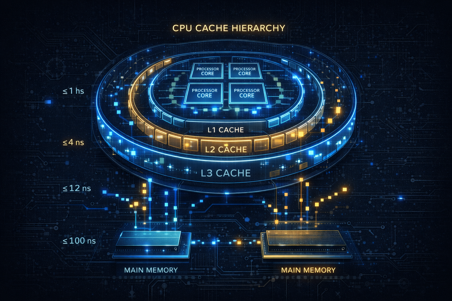
1.3 The Memory Hierarchy
Modern memory hierarchy (typical desktop/server):

                    Capacity    Latency      Bandwidth
┌─────────────┐
│  Registers  │     ~1 KB      0 cycles     Unlimited
└──────┬──────┘
       │
┌──────▼──────┐
│   L1 Cache  │     32-64 KB   3-4 cycles   ~1 TB/s
│  (per core) │     (split I/D)
└──────┬──────┘
       │
┌──────▼──────┐
│   L2 Cache  │     256 KB-1MB 10-12 cycles ~500 GB/s
│  (per core) │
└──────┬──────┘
       │
┌──────▼──────┐
│   L3 Cache  │     8-64 MB    30-50 cycles ~200 GB/s
│   (shared)  │
└──────┬──────┘
       │
┌──────▼──────┐
│  Main Memory│     16-256 GB  100-150 cyc  ~50 GB/s
│    (DRAM)   │
└──────┬──────┘
       │
┌──────▼──────┐
│   Storage   │     TB-PB      10⁵-10⁷ cyc  ~5 GB/s (NVMe)
│  (SSD/HDD)  │
└─────────────┘

Each level: ~10x larger, ~3-10x slower
Goal: Make memory appear as fast as L1, as large as disk
2. Cache Organization
How caches are structured internally.
2.1 Cache Lines
The fundamental unit of cache storage:

Cache line (typically 64 bytes):
┌────────────────────────────────────────────────────────┐
│  64 bytes of contiguous memory                         │
│  Address: 0x1000 - 0x103F                              │
│                                                        │
│  ┌──┬──┬──┬──┬──┬──┬──┬──┬──┬──┬──┬──┬──┬──┬──┬──┐    │
│  │B0│B1│B2│B3│B4│B5│B6│...                  │B63│    │
│  └──┴──┴──┴──┴──┴──┴──┴──┴──┴──┴──┴──┴──┴──┴──┴──┘    │
└────────────────────────────────────────────────────────┘

When you access one byte, entire 64-byte line is fetched:

int array[16];  // 64 bytes = 1 cache line

// This loop touches 1 cache line
for (int i = 0; i < 16; i++) {
    sum += array[i];
}

// First access: cache miss, fetch entire line
// Remaining 15 accesses: cache hits!

Address decomposition (example: 32KB L1, 8-way, 64-byte lines):
┌─────────────────┬──────────┬────────────┐
│      Tag        │   Index  │   Offset   │
│   (remaining)   │  (6 bits)│  (6 bits)  │
└─────────────────┴──────────┴────────────┘
                      64         64 bytes
                     sets       per line

Offset: Which byte within the cache line (log₂(64) = 6 bits)
Index: Which cache set (log₂(sets) bits)
Tag: Remaining bits to identify specific memory address
2.2 Cache Associativity
How cache lines are organized into sets:

Direct-mapped (1-way associative):
┌────────────────────────────────────────────────────────┐
│  Each memory address maps to exactly one cache line    │
│                                                        │
│  Set 0: [Line] ← Address 0x000, 0x100, 0x200 all map  │
│  Set 1: [Line]   here → conflicts!                     │
│  Set 2: [Line]                                         │
│  ...                                                   │
│                                                        │
│  Problem: Conflict misses when 2 addresses map to      │
│  same line and are accessed alternately                │
└────────────────────────────────────────────────────────┘

N-way set associative:
┌────────────────────────────────────────────────────────┐
│  Each address can go in any of N lines in a set       │
│                                                        │
│  8-way set associative (typical L1):                  │
│  Set 0: [L][L][L][L][L][L][L][L]  ← 8 choices         │
│  Set 1: [L][L][L][L][L][L][L][L]                      │
│  Set 2: [L][L][L][L][L][L][L][L]                      │
│  ...                                                   │
│                                                        │
│  Reduces conflict misses, but requires comparing       │
│  multiple tags in parallel                             │
└────────────────────────────────────────────────────────┘

Fully associative:
┌────────────────────────────────────────────────────────┐
│  Any address can go anywhere                           │
│  [L][L][L][L][L][L][L][L][L][L][L][L]...              │
│                                                        │
│  Best hit rate, but expensive:                         │
│  - Must compare tag against ALL lines                  │
│  - Used for small caches (TLB, victim cache)          │
└────────────────────────────────────────────────────────┘

Trade-offs:
             │ Direct │ 4-way │ 8-way │ Full
─────────────┼────────┼───────┼───────┼──────
Hit rate     │  Low   │ Good  │ Better│ Best
Complexity   │  Low   │ Medium│ Medium│ High
Power        │  Low   │ Medium│ Medium│ High
Latency      │  Low   │ Low   │ Low   │ High
2.3 Cache Parameters Example
Intel Core i7 (typical):

L1 Data Cache (per core):
- Size: 32 KB
- Associativity: 8-way
- Line size: 64 bytes
- Sets: 32KB / (8 ways × 64 bytes) = 64 sets
- Latency: 4 cycles

L1 Instruction Cache (per core):
- Size: 32 KB
- Associativity: 8-way
- Line size: 64 bytes
- Latency: 4 cycles

L2 Cache (per core):
- Size: 256 KB
- Associativity: 4-way
- Line size: 64 bytes
- Sets: 256KB / (4 × 64) = 1024 sets
- Latency: 12 cycles

L3 Cache (shared):
- Size: 8-32 MB
- Associativity: 16-way
- Line size: 64 bytes
- Latency: 40-50 cycles

View your CPU's cache:
$ lscpu | grep -i cache
$ cat /sys/devices/system/cpu/cpu0/cache/index0/size
$ getconf -a | grep CACHE
3. Cache Operations
What happens on reads and writes.
3.1 Cache Hits and Misses
Read hit:
┌─────────────────────────────────────────────────────────┐
│  CPU requests address 0x1234                            │
│                                                         │
│  1. Extract index and tag from address                 │
│  2. Look up set using index                            │
│  3. Compare tag with all tags in set                   │
│  4. Tag match found! → Return data                     │
│                                                         │
│  Time: 3-4 cycles (L1)                                 │
└─────────────────────────────────────────────────────────┘

Read miss:
┌─────────────────────────────────────────────────────────┐
│  CPU requests address 0x5678                            │
│                                                         │
│  1. Look up in L1 → Miss                               │
│  2. Look up in L2 → Miss                               │
│  3. Look up in L3 → Miss                               │
│  4. Fetch from memory (100+ cycles)                    │
│  5. Install in L3, L2, L1                              │
│  6. Return data to CPU                                 │
│                                                         │
│  Time: 100-150+ cycles                                 │
└─────────────────────────────────────────────────────────┘

Types of cache misses:

Compulsory (cold) miss:
- First access to data, never been in cache
- Unavoidable (except by prefetching)

Capacity miss:
- Working set larger than cache
- Data was evicted to make room for other data

Conflict miss:
- Two addresses map to same cache set
- Thrashing between them evicts each other
- Avoided by higher associativity
3.2 Write Policies
Write-through:
┌─────────────────────────────────────────────────────────┐
│  Write goes to both cache AND memory immediately       │
│                                                         │
│  CPU writes 0x42 to address 0x1000                     │
│  ├─► Update cache line                                 │
│  └─► Write to memory (or write buffer)                 │
│                                                         │
│  Pros: Memory always up-to-date, simple                │
│  Cons: Slow (every write hits memory)                  │
│                                                         │
│  Used in: Some L1 caches, embedded systems             │
└─────────────────────────────────────────────────────────┘

Write-back:
┌─────────────────────────────────────────────────────────┐
│  Write only updates cache, memory updated later        │
│                                                         │
│  CPU writes 0x42 to address 0x1000                     │
│  ├─► Update cache line                                 │
│  └─► Mark line as "dirty"                              │
│                                                         │
│  On eviction (if dirty):                               │
│  └─► Write entire line back to memory                  │
│                                                         │
│  Pros: Fast writes, less memory traffic                │
│  Cons: Complex, memory may be stale                    │
│                                                         │
│  Used in: Most L1/L2/L3 caches                         │
└─────────────────────────────────────────────────────────┘

Write-allocate vs no-write-allocate:

Write-allocate (write miss → fetch line, then write):
- Good for subsequent reads/writes to same line
- Used with write-back

No-write-allocate (write miss → write directly to memory):
- Good for write-once data
- Used with write-through
3.3 Replacement Policies
When cache set is full, which line to evict?

LRU (Least Recently Used):
┌─────────────────────────────────────────────────────────┐
│  Track access order, evict oldest                       │
│                                                         │
│  Access sequence: A, B, C, D, A, E                     │
│  4-way set, all full, need to add E                    │
│                                                         │
│  Before: [A:2] [B:1] [C:0] [D:3]  (numbers = recency)  │
│  A accessed: [A:3] [B:1] [C:0] [D:2]                   │
│  Evict C (oldest): [A:3] [B:1] [E:4] [D:2]            │
│                                                         │
│  Pros: Good hit rate                                   │
│  Cons: Expensive to track exactly                      │
└─────────────────────────────────────────────────────────┘

Pseudo-LRU:
- Approximate LRU with less state
- Tree-based or bit-based tracking
- Most L1/L2 caches use this

Random:
- Simple, no tracking needed
- Surprisingly effective for larger caches
- Sometimes used in L3

RRIP (Re-Reference Interval Prediction):
- Modern policy, predicts re-use distance
- Handles scan patterns better than LRU
- Used in recent Intel CPUs
4. Cache Coherence
Keeping multiple caches consistent in multicore systems.
4.1 The Coherence Problem
Multiple cores, each with private caches:

Core 0              Core 1              Core 2
┌────────┐         ┌────────┐          ┌────────┐
│  L1    │         │  L1    │          │  L1    │
│ X = 5  │         │ X = 5  │          │ X = ?  │
└────┬───┘         └────┬───┘          └────┬───┘
     │                  │                   │
     └──────────────────┼───────────────────┘
                        │
                   ┌────▼────┐
                   │   L3    │
                   │ (shared)│
                   └────┬────┘
                        │
                   ┌────▼────┐
                   │  Memory │
                   │  X = 5  │
                   └─────────┘

Problem scenario:
1. Core 0 reads X = 5 (cached in L1)
2. Core 1 reads X = 5 (cached in L1)
3. Core 0 writes X = 10 (only updates own L1!)
4. Core 1 reads X → Gets stale value 5!

This is the cache coherence problem.
4.2 MESI Protocol
MESI: Cache line states for coherence

┌────────────┬───────────────────────────────────────────┐
│   State    │   Meaning                                  │
├────────────┼───────────────────────────────────────────┤
│ Modified   │ Line is dirty, only copy, must write back│
│ Exclusive  │ Line is clean, only copy, can modify     │
│ Shared     │ Line is clean, other copies may exist    │
│ Invalid    │ Line is not valid, must fetch            │
└────────────┴───────────────────────────────────────────┘

State transitions:

Read by Core 0 (line not in any cache):
Memory → Core 0 (Exclusive)

Read by Core 1 (line Exclusive in Core 0):
Core 0 (Exclusive → Shared), Core 1 (Shared)

Write by Core 0 (line Shared):
Core 0 (Shared → Modified)
Core 1 (Shared → Invalid)  ← Invalidation message!

Write by Core 0 (line Modified in Core 1):
Core 1 writes back to memory (Modified → Invalid)
Core 0 fetches and modifies (→ Modified)

┌──────────────────────────────────────────────────────────┐
│              MESI State Diagram                          │
│                                                          │
│              ┌─────────┐                                 │
│              │ Invalid │◄────────────────────────┐      │
│              └────┬────┘                         │      │
│      Read miss    │                     Other    │      │
│      (exclusive)  │                     writes   │      │
│                   ▼                              │      │
│              ┌─────────┐      Read by           │      │
│        ┌────►│Exclusive│──────other────►┌───────┴──┐   │
│        │     └────┬────┘      core      │  Shared  │   │
│        │          │                      └────┬─────┘   │
│        │   Local  │                           │        │
│        │   write  │                      Local│        │
│        │          ▼                      write│        │
│        │     ┌─────────┐                      │        │
│        └─────┤Modified │◄─────────────────────┘        │
│   Eviction   └─────────┘                               │
│   (write back)                                          │
└──────────────────────────────────────────────────────────┘
4.3 Cache Coherence Traffic
Coherence has performance implications:

False sharing:
┌─────────────────────────────────────────────────────────┐
│  Two cores write to different variables, same line      │
│                                                         │
│  struct { int counter0; int counter1; } counters;      │
│  // Both fit in one 64-byte cache line!                │
│                                                         │
│  Core 0: counter0++  → Invalidates entire line         │
│  Core 1: counter1++  → Must fetch line, invalidates    │
│  Core 0: counter0++  → Must fetch line, invalidates    │
│  ...ping-pong continues...                             │
│                                                         │
│  Solution: Pad to separate cache lines                 │
│  struct alignas(64) { int counter; char pad[60]; };    │
└─────────────────────────────────────────────────────────┘

Coherence bandwidth:
- Invalidation messages consume interconnect bandwidth
- Write-heavy workloads generate traffic
- Monitor with perf: cache coherence events

Snoop traffic:
- Every cache monitors (snoops) bus for relevant addresses
- Scales poorly with core count
- Modern CPUs use directory-based coherence for L3
4.4 Memory Ordering and Barriers
Caches complicate memory ordering:

CPU reordering:
- CPUs may reorder memory operations for performance
- Writes may appear out-of-order to other cores
- Store buffers delay visibility of writes

Example problem:
// Initially: x = 0, y = 0

Core 0:              Core 1:
x = 1;               y = 1;
r0 = y;              r1 = x;

// Possible result: r0 = 0, r1 = 0!
// Both reads happened before either write became visible

Memory barriers force ordering:
x = 1;
__sync_synchronize();  // Full barrier
r0 = y;

// Now: x = 1 is visible before reading y

Barrier types:
- Load barrier: Previous loads complete before following loads
- Store barrier: Previous stores complete before following stores
- Full barrier: All operations complete before crossing

C11/C++11 memory model:
std::atomic<int> x;
x.store(1, std::memory_order_release);  // Release barrier
r = x.load(std::memory_order_acquire);  // Acquire barrier
5. Performance Implications
How cache behavior affects real code.
5.1 Cache-Friendly Code
Good: Sequential access pattern
┌─────────────────────────────────────────────────────────┐
│  // Row-major order (C layout)                          │
│  int matrix[1000][1000];                               │
│                                                         │
│  // Cache-friendly: sequential in memory               │
│  for (int i = 0; i < 1000; i++)                        │
│      for (int j = 0; j < 1000; j++)                    │
│          sum += matrix[i][j];                          │
│                                                         │
│  Memory layout: [0,0][0,1][0,2]...[0,999][1,0][1,1]... │
│  Access pattern matches layout → excellent locality    │
└─────────────────────────────────────────────────────────┘

Bad: Strided access pattern
┌─────────────────────────────────────────────────────────┐
│  // Column-major access in row-major array             │
│  for (int j = 0; j < 1000; j++)                        │
│      for (int i = 0; i < 1000; i++)                    │
│          sum += matrix[i][j];                          │
│                                                         │
│  Access: [0,0] then [1,0] (4000 bytes apart!)          │
│  Each access likely a cache miss                       │
│  Can be 10-100x slower than row-major traversal        │
└─────────────────────────────────────────────────────────┘

Performance comparison (typical):
Pattern              │ L1 hits  │ Cycles/element
─────────────────────┼──────────┼───────────────
Sequential           │  97%     │  ~1
Stride 16 bytes      │  75%     │  ~3
Stride 64 bytes      │  25%     │  ~10
Stride 4096 bytes    │  ~0%     │  ~50+
Random               │  ~0%     │  ~100+
5.2 Data Structure Layout
Array of Structures (AoS) vs Structure of Arrays (SoA):

AoS (traditional):
struct Particle {
    float x, y, z;      // Position: 12 bytes
    float vx, vy, vz;   // Velocity: 12 bytes
    float mass;         // Mass: 4 bytes
    int id;             // ID: 4 bytes
};                      // Total: 32 bytes
Particle particles[1000];

// Processing positions loads velocity, mass, id too
for (int i = 0; i < 1000; i++) {
    particles[i].x += dt * particles[i].vx;
    // Cache line contains: x,y,z,vx,vy,vz,mass,id
    // Only using x and vx = 25% utilization
}

SoA (cache-friendly for specific operations):
struct Particles {
    float x[1000];
    float y[1000];
    float z[1000];
    float vx[1000];
    float vy[1000];
    float vz[1000];
    float mass[1000];
    int id[1000];
};

// Now position update only loads positions and velocities
for (int i = 0; i < 1000; i++) {
    particles.x[i] += dt * particles.vx[i];
    // Cache lines contain: only x values (or only vx values)
    // 100% utilization for this operation
}

Hybrid AoSoA:
struct ParticleBlock {
    float x[8], y[8], z[8];     // 8 particles' positions
    float vx[8], vy[8], vz[8];  // 8 particles' velocities
};
// Balances locality with SIMD-friendly layout
5.3 Cache Blocking (Tiling)
Matrix multiplication without blocking:

// Naive: terrible cache performance for large matrices
for (int i = 0; i < N; i++)
    for (int j = 0; j < N; j++)
        for (int k = 0; k < N; k++)
            C[i][j] += A[i][k] * B[k][j];

// B accessed column-wise → cache misses
// For 1000x1000 matrix: ~1 billion cache misses!

With cache blocking:
┌─────────────────────────────────────────────────────────┐
│  #define BLOCK 64  // Fits in L1 cache                 │
│                                                         │
│  for (int i0 = 0; i0 < N; i0 += BLOCK)                 │
│    for (int j0 = 0; j0 < N; j0 += BLOCK)               │
│      for (int k0 = 0; k0 < N; k0 += BLOCK)             │
│        // Process BLOCK × BLOCK submatrices            │
│        for (int i = i0; i < min(i0+BLOCK, N); i++)     │
│          for (int j = j0; j < min(j0+BLOCK, N); j++)   │
│            for (int k = k0; k < min(k0+BLOCK, N); k++) │
│              C[i][j] += A[i][k] * B[k][j];             │
└─────────────────────────────────────────────────────────┘

Why it works:
- Submatrices fit in cache
- Process entire block before moving on
- Reuse cached data maximally

Performance improvement: Often 5-10x for large matrices
5.4 Prefetching
Hardware prefetching:
- CPU detects sequential access patterns
- Fetches next cache lines before needed
- Works great for arrays, fails for pointer chasing

Software prefetching:
┌─────────────────────────────────────────────────────────┐
│  // Prefetch hint for future access                    │
│  for (int i = 0; i < N; i++) {                         │
│      __builtin_prefetch(&data[i + 16], 0, 3);         │
│      // 0 = read, 3 = high temporal locality           │
│      process(data[i]);                                 │
│  }                                                     │
│                                                         │
│  // Or with intrinsics                                 │
│  _mm_prefetch(&data[i + 16], _MM_HINT_T0);            │
└─────────────────────────────────────────────────────────┘

When software prefetch helps:
- Irregular access patterns (linked lists, trees)
- Known future access (graph algorithms)
- Latency hiding in compute-bound code

When it hurts:
- Already in cache (wasted bandwidth)
- Too late (data needed immediately)
- Too early (evicted before use)
- Too many prefetches (cache pollution)

Prefetch distance = memory_latency / time_per_iteration
Example: 200 cycles latency, 10 cycles/iter → prefetch 20 ahead
6. Measuring Cache Performance
Tools and techniques for cache analysis.
6.1 Performance Counters
# Linux perf for cache statistics
perf stat -e cache-references,cache-misses,L1-dcache-loads,\
L1-dcache-load-misses,LLC-loads,LLC-load-misses ./program

# Example output:
# 1,234,567 cache-references
#   123,456 cache-misses              #    10% of all refs
# 5,678,901 L1-dcache-loads
#   234,567 L1-dcache-load-misses     #     4.1% of all L1 loads
#   345,678 LLC-loads
#    34,567 LLC-load-misses           #    10% of all LLC loads

# Record and analyze
perf record -e cache-misses ./program
perf report

# Compare implementations
perf stat -e cycles,L1-dcache-load-misses ./version1
perf stat -e cycles,L1-dcache-load-misses ./version2
6.2 Cachegrind
# Valgrind's cache simulator
valgrind --tool=cachegrind ./program

# Output:
# I   refs:      1,234,567
# I1  misses:        1,234
# LLi misses:          123
# I1  miss rate:      0.1%
# LLi miss rate:      0.01%
#
# D   refs:        567,890  (345,678 rd + 222,212 wr)
# D1  misses:       12,345  (  8,901 rd +   3,444 wr)
# LLd misses:        1,234  (    890 rd +     344 wr)
# D1  miss rate:      2.2%  (    2.6%   +     1.5%  )
# LLd miss rate:      0.2%  (    0.3%   +     0.2%  )

# Annotated source code
cg_annotate cachegrind.out.12345

# Compare runs
cg_diff cachegrind.out.v1 cachegrind.out.v2
6.3 Cache-Aware Benchmarking
// Measure memory bandwidth at different sizes
void benchmark_cache_levels() {
    for (size_t size = 1024; size <= 256*1024*1024; size *= 2) {
        char *buffer = malloc(size);

        // Warmup
        memset(buffer, 0, size);

        clock_t start = clock();
        for (int iter = 0; iter < 100; iter++) {
            for (size_t i = 0; i < size; i += 64) {
                buffer[i]++;  // Touch each cache line
            }
        }
        clock_t end = clock();

        double time = (double)(end - start) / CLOCKS_PER_SEC;
        double bandwidth = (size * 100.0) / time / 1e9;
        printf("Size: %8zu KB, Bandwidth: %.2f GB/s\n",
               size/1024, bandwidth);

        free(buffer);
    }
}

// You'll see bandwidth drop at L1, L2, L3 boundaries:
// Size:        1 KB, Bandwidth: 85.2 GB/s  (L1)
// Size:       32 KB, Bandwidth: 82.1 GB/s  (L1)
// Size:       64 KB, Bandwidth: 45.3 GB/s  (L2)
// Size:      256 KB, Bandwidth: 42.8 GB/s  (L2)
// Size:      512 KB, Bandwidth: 28.5 GB/s  (L3)
// Size:     8192 KB, Bandwidth: 25.1 GB/s  (L3)
// Size:    16384 KB, Bandwidth: 12.3 GB/s  (Memory)
6.4 Intel VTune and AMD uProf
Advanced profiling tools:

Intel VTune Profiler:
- Memory Access analysis
- Cache-to-DRAM bandwidth
- Per-line cache miss attribution
- Microarchitecture exploration

vtune -collect memory-access ./program
vtune -report hotspots -r r000ma

AMD uProf:
- Similar capabilities for AMD CPUs
- L1/L2/L3 miss analysis
- Memory bandwidth analysis

Key metrics to examine:
- Cache miss rate per function
- Memory bandwidth utilization
- Cache line utilization (bytes used per line fetched)
- False sharing detection
7. Advanced Cache Topics
Modern cache features and optimizations.
7.1 Non-Temporal Stores
Bypassing cache for write-once data:

Normal store:
write(addr) → Allocate cache line → Write to cache → Eventually write back

Problem: If data won't be read soon, cache space is wasted

Non-temporal (streaming) store:
write(addr) → Write directly to memory, bypass cache

// SSE/AVX intrinsics
_mm_stream_si128((__m128i*)ptr, value);  // 16 bytes
_mm256_stream_si256((__m256i*)ptr, value);  // 32 bytes

// Must combine writes to fill write-combine buffer
// Use _mm_sfence() after streaming stores

Use cases:
- Memset/memcpy of large buffers
- Writing output that won't be read
- GPU data uploads
- Avoiding cache pollution
7.2 Hardware Transactional Memory
Intel TSX / AMD equivalent:

Transactional execution using cache:
┌─────────────────────────────────────────────────────────┐
│  if (_xbegin() == _XBEGIN_STARTED) {                   │
│      // Transaction body                                │
│      counter++;                                         │
│      linked_list_insert(item);                         │
│      _xend();  // Commit                               │
│  } else {                                              │
│      // Fallback to locks                              │
│      mutex_lock(&lock);                                │
│      counter++;                                         │
│      linked_list_insert(item);                         │
│      mutex_unlock(&lock);                              │
│  }                                                     │
└─────────────────────────────────────────────────────────┘

How it works:
- Cache tracks read/write sets
- On conflict (another core touches same line): abort
- On commit: atomically make changes visible

Limitations:
- Aborts on cache eviction (large transactions fail)
- Some instructions cause abort
- Need fallback path
7.3 Cache Partitioning
Intel Cache Allocation Technology (CAT):

Divide L3 cache among applications:
┌─────────────────────────────────────────────────────────┐
│  L3 Cache (20 MB, 20 ways)                             │
│                                                         │
│  Ways: |0|1|2|3|4|5|6|7|8|9|A|B|C|D|E|F|G|H|I|J|       │
│        └──────────┘ └────────────────────────┘         │
│         Latency-    Throughput application             │
│         sensitive   (gets 16 ways = 16 MB)             │
│         app (4 ways)                                   │
└─────────────────────────────────────────────────────────┘

Use cases:
- Isolate noisy neighbors in cloud
- Guarantee cache for latency-sensitive workloads
- Prevent cache thrashing between containers

# Configure with Linux resctrl
mount -t resctrl resctrl /sys/fs/resctrl
echo "L3:0=f" > /sys/fs/resctrl/schemata  # Ways 0-3
echo $PID > /sys/fs/resctrl/tasks
7.4 NUMA and Cache Considerations
Non-Uniform Memory Access with caches:

NUMA topology:
┌─────────────────────┐     ┌─────────────────────┐
│     Socket 0        │     │     Socket 1        │
│  ┌──────┐ ┌──────┐  │     │  ┌──────┐ ┌──────┐  │
│  │Core 0│ │Core 1│  │     │  │Core 4│ │Core 5│  │
│  │ L1/2 │ │ L1/2 │  │     │  │ L1/2 │ │ L1/2 │  │
│  └──┬───┘ └───┬──┘  │     │  └──┬───┘ └───┬──┘  │
│     └────┬────┘     │     │     └────┬────┘     │
│      ┌───▼───┐      │     │      ┌───▼───┐      │
│      │  L3   │      │◄═══►│      │  L3   │      │
│      └───┬───┘      │ QPI │      └───┬───┘      │
│      ┌───▼───┐      │     │      ┌───▼───┐      │
│      │Memory │      │     │      │Memory │      │
│      │Node 0 │      │     │      │Node 1 │      │
│      └───────┘      │     │      └───────┘      │
└─────────────────────┘     └─────────────────────┘

Memory access latencies:
- Local L3: 40 cycles
- Remote L3: 80-100 cycles (cross-socket snoop)
- Local memory: 100 cycles
- Remote memory: 150-200 cycles

Cache coherence across sockets:
- L3 miss may snoop remote L3
- Remote cache hit still faster than remote memory
- But coherence traffic adds latency

Optimization:
- Allocate memory on local node
- Bind threads to cores near their data
- Minimize cross-socket sharing
8. Cache-Aware Algorithms
Designing algorithms with cache in mind.
8.1 Cache-Oblivious Algorithms
Work well regardless of cache parameters:

Cache-oblivious matrix transpose:
┌─────────────────────────────────────────────────────────┐
│  void transpose(int *A, int *B, int n,                 │
│                 int rb, int re, int cb, int ce) {      │
│      int rows = re - rb;                               │
│      int cols = ce - cb;                               │
│                                                         │
│      if (rows <= THRESHOLD && cols <= THRESHOLD) {     │
│          // Base case: direct transpose                │
│          for (int i = rb; i < re; i++)                 │
│              for (int j = cb; j < ce; j++)             │
│                  B[j*n + i] = A[i*n + j];              │
│      } else if (rows >= cols) {                        │
│          // Split rows                                 │
│          int mid="rb" + rows/2;                        │
│          transpose(A, B, n, rb, mid, cb, ce);          │
│          transpose(A, B, n, mid, re, cb, ce);          │
│      } else {                                          │
│          // Split columns                              │
│          int mid="cb" + cols/2;                        │
│          transpose(A, B, n, rb, re, cb, mid);          │
│          transpose(A, B, n, rb, re, mid, ce);          │
│      }                                                 │
│  }                                                     │
└─────────────────────────────────────────────────────────┘

Why it works:
- Recursively divides until subproblem fits in cache
- No need to know cache size
- Automatically adapts to all cache levels
8.2 B-Trees for Cache Efficiency
B-trees are cache-aware data structures:

Binary search tree (cache-unfriendly):
┌─────┐
│  8  │ ← Each node = separate allocation
├──┬──┤
│  │  │
▼  ▼  ▼
4    12   ← Random memory locations
...       ← Pointer chasing = cache misses

B-tree with node size = cache line:
┌──────────────────────────────────────────┐
│  [3] [5] [8] [12] [15] [20] [25] ...    │ ← One cache line
│   │   │   │   │    │    │    │          │   All keys together
└───┼───┼───┼───┼────┼────┼────┼──────────┘
    ▼   ▼   ▼   ▼    ▼    ▼    ▼
   Children (also full cache lines)

Benefits:
- One cache miss per tree level
- 10+ keys per node vs 1 for binary tree
- log_B(N) misses vs log_2(N)
- For B=16, 16^3 = 4096 keys in 3 cache misses
8.3 Cache-Efficient Sorting
Merge sort with cache awareness:

Standard merge sort:
- Recurses down to single elements
- Merges across entire array
- Poor cache utilization during merge

Cache-aware merge sort:
┌─────────────────────────────────────────────────────────┐
│  void cache_aware_sort(int *arr, int n) {              │
│      // Sort cache-sized chunks with insertion sort    │
│      // (good for small, cache-resident data)          │
│      for (int i = 0; i < n; i += CACHE_SIZE) {         │
│          int end = min(i + CACHE_SIZE, n);             │
│          insertion_sort(arr + i, end - i);             │
│      }                                                 │
│                                                         │
│      // Merge sorted chunks                            │
│      // Use multi-way merge to reduce passes           │
│      multiway_merge(arr, n, CACHE_SIZE);               │
│  }                                                     │
└─────────────────────────────────────────────────────────┘

Radix sort for cache efficiency:
- MSD radix sort: cache-oblivious partitioning
- LSD radix sort: sequential writes (streaming)
- Good when data fits sort assumptions
9. Practical Optimization Strategies
Applying cache knowledge to real problems.
9.1 Common Optimization Patterns
1. Loop reordering:
// Before: Column-major access in row-major array
for (j = 0; j < N; j++)
    for (i = 0; i < N; i++)
        a[i][j] = ...;

// After: Row-major access
for (i = 0; i < N; i++)
    for (j = 0; j < N; j++)
        a[i][j] = ...;

2. Loop fusion:
// Before: Two passes over data
for (i = 0; i < N; i++) a[i] = b[i] * 2;
for (i = 0; i < N; i++) c[i] = a[i] + 1;

// After: One pass, data still in cache
for (i = 0; i < N; i++) {
    a[i] = b[i] * 2;
    c[i] = a[i] + 1;
}

3. Data packing:
// Before: Array of pointers (indirection)
Object **ptrs;
for (i = 0; i < N; i++) process(ptrs[i]);

// After: Contiguous array
Object objs[N];
for (i = 0; i < N; i++) process(&objs[i]);
9.2 Alignment Considerations
Cache line alignment:

// Ensure structure starts on cache line boundary
struct alignas(64) CacheAligned {
    int counter;
    char padding[60];  // Fill rest of cache line
};

// Allocate aligned memory
void *ptr = aligned_alloc(64, size);

// Check alignment
assert(((uintptr_t)ptr & 63) == 0);

Why alignment matters:
┌─────────────────────────────────────────────────────────┐
│  Unaligned access (straddles two lines):               │
│                                                         │
│  Cache line N:   [.......████]                         │
│  Cache line N+1: [████........]                        │
│                   └──────┘                             │
│                   One access = two cache lines!        │
│                                                         │
│  Aligned access:                                       │
│  Cache line N:   [████████....]                        │
│                   One access = one cache line          │
└─────────────────────────────────────────────────────────┘
9.3 Working Set Analysis
Understanding your working set:

Phases of execution:
┌─────────────────────────────────────────────────────────┐
│  Phase 1 (Init): Working set = 10 KB → fits in L1     │
│  Phase 2 (Main): Working set = 2 MB → fits in L3      │
│  Phase 3 (Merge): Working set = 50 MB → memory-bound  │
└─────────────────────────────────────────────────────────┘

Measuring working set:
1. Run with increasing array sizes
2. Find where performance drops
3. That's your cache level boundary

Reducing working set:
- Smaller data types (int16 vs int32 vs int64)
- Bit packing for flags
- Compression for cold data
- Process in cache-sized chunks
- Stream processing instead of random access
10. Summary and Guidelines
Condensed wisdom for cache-aware programming.
10.1 Key Takeaways
Cache fundamentals:
✓ Memory is slow, cache is fast
✓ Cache works on 64-byte lines
✓ Locality (temporal and spatial) is key
✓ Working set size determines cache effectiveness

Performance rules:
✓ Sequential access beats random access
✓ Smaller data beats larger data
✓ Hot data together, cold data separate
✓ Avoid false sharing in multithreaded code
✓ Measure before and after optimizing

Architecture awareness:
✓ Know your cache sizes (L1: 32KB, L2: 256KB, L3: 8-32MB)
✓ Know your cache line size (64 bytes)
✓ Know cache miss latency (L1: 4, L2: 12, L3: 40, Mem: 100+)
✓ Use performance counters to validate assumptions
10.2 Optimization Checklist
When optimizing for cache:

□ Profile first (perf stat, cachegrind)
□ Identify hot loops and data structures
□ Check access patterns (sequential vs random)
□ Measure cache miss rates
□ Consider data layout (AoS vs SoA)
□ Apply loop transformations if needed
□ Use blocking for large working sets
□ Align data to cache lines when appropriate
□ Avoid false sharing in parallel code
□ Consider prefetching for irregular access
□ Test with realistic data sizes
□ Verify improvement with benchmarks
□ Document cache-sensitive code sections
□ Monitor for regressions over time
The cache hierarchy stands as one of the most successful abstractions in computer architecture, making fast memory appear both large and accessible while hiding the physical realities of distance and latency. From the earliest CPUs with simple caches to modern processors with sophisticated multilevel hierarchies, coherence protocols, and predictive prefetchers, the principles remain constant: exploit locality, minimize misses, and keep the CPU fed with data. Whether you’re optimizing tight numerical kernels or designing large-scale data systems, understanding how your code interacts with the cache hierarchy reveals optimization opportunities invisible to those who see memory as a uniform flat address space. The cache is not just a performance feature but a fundamental aspect of how modern computers operate and achieve their remarkable speeds.