CPU Microarchitecture: Pipelines, Out-of-Order Execution, and Modern Performance

2025-12-04 · Leonardo Benicio

An in-depth exploration of CPU microarchitecture: instruction pipelines, hazards, branch prediction, out-of-order execution, register renaming, superscalar and SIMD units, and how software maps to hardware for performance.

Modern CPUs are marvels of engineering designed to extract instruction-level parallelism (ILP) from sequential programs while hiding long latencies — memory, multiplies, or long dependency chains. To understand why some code runs orders of magnitude faster than other code that “does the same work,” you need to understand microarchitectural components such as pipelines, superscalar issue, branch prediction, out-of-order (OoO) execution, register renaming, reorder buffers, and vector (SIMD) units. This article takes a practical tour of these features, how they affect instruction throughput and latency, and pragmatic tips for writing high-performance code.

1. The instruction pipeline: stages and hazards

CPUs break instruction processing into stages to increase throughput (instructions per cycle — IPC) by working on several instructions simultaneously.

Typical pipeline stages:

Fetch: Read instruction bytes from the instruction cache (I-cache).
Decode: Convert instruction bytes into internal micro-operations (uops).
Rename: Map architectural registers to physical registers (for OoO).
Issue/Dispatch: Place ready uops into reservation stations or issue queues.
Execute: Perform ALU, load/store, branch, or vector operations in execution units.
Writeback: Write results to physical registers or store buffers.
Retire/Commit: Architecturally commit instruction results and free resources.

Pipelining increases throughput but introduces hazards — conditions that prevent the next instruction in the pipeline from executing in the next cycle.

Hazard types:

Structural hazards: Two instructions require the same hardware resource (e.g., a single ALU port).
Data hazards: Instruction depends on the result of a prior instruction. Types: RAW (read after write), WAR, WAW.
Control hazards: Branches and jumps that change the flow of control.

Mitigation strategies include deeper pipelines, forwarding (bypassing), register renaming, and speculative execution.

1.1 Pipeline bubbles and stalls

A pipeline bubble occurs when a stage cannot proceed, leaving a gap that wastes cycles. Causes include cache misses (long latency), dependencies causing stalls, and branch mispredictions requiring pipeline flushes. A key optimization goal is keeping the pipeline full.

1.2 Example: simple 5-stage pipeline

Classic RISC 5-stage pipeline (IF/ID/EX/MEM/WB) shows the basic ideas. With forwarding, many RAW hazards can be resolved without stalls; but load-use hazards (load followed by use) often require a one-cycle stall if the load value isn’t available early enough.

2. Superscalar and instruction-level parallelism (ILP)

A superscalar processor can issue multiple instructions per cycle (e.g., 4-wide, 8-wide), extracting ILP dynamically.

Key challenges:

Dependence analysis: The hardware must detect which instructions can execute in parallel.
Resource allocation: Multiple functional units (ALUs, FPUs, load/store units) must be scheduled without conflicts.

Programmers can increase ILP by writing code with many independent operations, avoiding long chains of serial dependencies, and using vector instructions where possible.

3. Branch prediction and control speculation

Branches are the main source of control hazards. Modern CPUs use powerful branch predictors to guess the outcome and speculatively execute down the predicted path.

Components:

Branch Target Buffer (BTB): Predicts the target address of taken branches.
Branch history: Global and local history tables track patterns of taken/not-taken outcomes.
Return Stack Buffer (RSB): Predicts return addresses for call/ret sequences (LIFO behavior).
Indirect branch prediction: Special mechanisms for indirect/jump-table branches (important for virtual calls).

3.1 Static vs dynamic predictors

Static predictors: e.g., always not taken or predict backward-taken/forward-not-taken; simple but ineffective for general code.
Dynamic predictors: Use runtime history and pattern tables to adapt to branches’ behavior. Common dynamic schemes:
- 2-bit saturating counters: A 2-bit counter per branch gives hysteresis (strong/weak taken/not-taken).
- Local history: Per-branch local history registers (LHR) with local pattern tables capture branch-specific patterns.
- Global history (gshare, global PHT): XOR global history with branch address to index pattern history tables, capturing correlation between branches.
- Tournament predictors: Combine local and global predictors and use a chooser to pick the best predictor for each branch.
- TAGE (TAgged GEometric history) and perceptron predictors: Modern, highly accurate predictors that use multiple history lengths or simple linear models (perceptron) to capture complex patterns.

3.1.1 Indirect and return prediction

Return Stack Buffer (RSB): Captures call/return stack to predict return targets with LIFO behavior. RSB underflow/overflow can lead to mispredictions on deep call chains.
Indirect branch prediction: Specialized tables attempt to predict targets of indirect branches (virtual calls, jump tables); accuracy is crucial for JITs and OO-heavy code.

3.1.2 TAGE and perceptron predictors (advanced)

Modern high-performance predictors like TAGE (TAgged GEometric history) and perceptron-based predictors significantly outperform simple 2-bit or gshare predictors by using multiple history lengths and simple linear classifiers.

TAGE: Maintains several tables indexed by different history lengths (geometric series). If a match is found in a longer history table, the predictor uses that entry; otherwise it falls back to shorter histories. This adapts to patterns of different spans and achieves very high accuracy.
Perceptron predictors: Treat prediction as a dot product between weights and global history bits; they are able to learn linearly separable patterns and reduce aliasing in some workloads. Perceptrons are heavier in hardware but improve accuracy for complex correlations.

Design trade-offs:

Storage vs accuracy: Larger tables and more history lengths increase accuracy but cost silicon area and power.
Update cost: Sophisticated predictors require more logic on misprediction to update weights or tags.

Implications for developers:

Certain code idioms (indirect dispatch loops, alternating patterns) still cause mispredictions; minimizing unpredictable indirect branches or optimizing callsite locality helps.

3.2 Misprediction penalty

If a branch is mispredicted, the pipeline must flush speculative instructions and fetch from the correct path; the penalty equals the pipeline depth plus any front-end delays. Techniques to reduce effective penalty:

Shorter pipelines: Easier recovery but lower clock frequency potential.
Early branch resolution: Some CPUs resolve certain branches earlier (e.g., simple condition checks in decode stage) to reduce penalty.
Speculative prefetch on predicted path to warm caches for the likely successor.

Practical tip: Measure branch-misses and correlate with stalled-cycles-frontend to assess whether mispredictions are the performance limiter.

Shorter pipelines: Easier recovery but lower clock frequency potential.
Early branch resolution: Some CPUs resolve certain branches earlier (e.g., simple condition checks in decode stage) to reduce penalty.
Speculative prefetch on predicted path to warm caches for the likely successor.

Practical tip: Measure branch-misses and correlate with stalled-cycles-frontend to assess whether mispredictions are the performance limiter.

If a branch is mispredicted, the pipeline must flush speculative instructions and fetch from the correct path; the penalty equals the depth of the pipeline plus any front-end delays. Deep pipelines and wide front-ends amplify the cost of misprediction.

3.3 Techniques to reduce mispredictions

Algorithmic changes: Reduce conditional branches (e.g., use arithmetic or predication if supported).
Branchless programming: Use conditional moves (CMOV) or select instructions.
Code layout: Place hot paths sequentially to improve static fall-through success.
Profile-guided optimization: Reorder code according to branch frequencies.

4. Out-of-Order execution and register renaming

To tolerate long latencies and exploit parallelism, modern processors execute instructions out-of-order while maintaining appearance of in-order execution via reorder buffers and register renaming.

4.1 Why OoO helps

Consider code that issues a cacheable load followed by independent arithmetic. With in-order execution, the CPU must wait for the load to complete before executing subsequent instructions, stalling the pipeline. With OoO, the CPU can execute independent instructions that are ready, keeping execution units busy while the load completes.

4.2 Register renaming

Architectural registers (e.g., eax, rbx) are limited and create false dependencies (WAR, WAW). Register renaming maps architectural registers to a larger pool of physical registers, eliminating false dependencies and enabling more parallelism.

Mechanism:

Rename table: Maps architectural reg → physical reg.
Free list: Physical registers available for allocation.
On rename, a new physical reg is assigned for the destination; source operands refer to currently mapped physical regs.
On retire, old physical regs are released back to free list.

4.3 Reorder Buffer (ROB) and retirement

The ROB holds instructions in program order until retirement, allowing speculative and out-of-order execution but guaranteeing in-order commit. On misprediction or exception, speculative instructions are undone by rolling back the rename map and freeing speculative registers.

4.4 Front-end and back-end microarchitecture (decoders, uop cache, ports)

Modern CPUs separate the front-end (fetch/decode/rename) from the back-end (issue/execute/retire) with multiple optimizations to improve throughput and hide latencies.

Front-end components:

I-cache and fetch bandwidth: The instruction cache supplies bytes to the instruction fetcher. The fetch width (bytes or instruction count per cycle) limits how many instructions can enter the pipeline.
Decode stage: For CISC ISAs like x86, decoders split complex instructions into micro-ops. Some CPUs have multiple simple decoders and one complex decoder.
Micro-op cache / trace cache: Caches decoded micro-ops to avoid re-decoding and improve fetch/decode throughput. Intel’s micro-op cache and loop stream detector are examples.
Branch predictor & BTB: Predict control flow to keep the pipeline supplied with fetch addresses.

Back-end components:

Issue queues / reservation stations: Hold decoded micro-ops until their operands are ready; wakeup/select logic chooses ready micro-ops to issue to execution ports.
Execution ports and units: Modern CPUs expose a set of ports (0..N) connected to ALUs, multipliers, vector units, and memory units. Scheduling maps micro-ops to ports depending on functional capability.
Physical register file: Stores renaming allocations and writeback results; ported to support multiple read/writes per cycle.
Store buffer & load queue: Hold pending memory operations; stores retire but remain buffered until written to L1/L2 caches.

Port model example (simplified): An Intel core might have ports 0/1 for ALU, port 2 for load, port 3 for store, port 5/6 for AVX ops; micro-ops map to available ports. Resource pressure or port conflicts can limit effective throughput.

Hardware-level metrics that reflect front-end/back-end health:

Frontend stalls / fetch bandwidth: If stalled-cycles-frontend is high, the front-end can’t feed the back-end (e.g., instruction cache misses or decode bottleneck).
Backend stalls / resource stalls: stalled-cycles-backend indicates execution or memory-bound stalls.
Retire width: The number of micro-ops retired per cycle — if retirement is the bottleneck, the CPI rises despite a busy execution engine.

Understanding both front-end and back-end limits helps identify whether a workload is decode-limited (complex instruction mix), fetch-limited (I-cache misses or branch mispredictions), port-limited (too many operations contending for the same port), or memory-limited (LLC misses and memory latency).

Optimization levers:

Reduce instruction working set (better I-cache locality, smaller code).
Replace complex instruction sequences by fused micro-op-friendly patterns.
Balance instruction mix across ports (e.g., avoid saturating a single ALU port).
Use micro-benchmarks to isolate front-end vs back-end bottlenecks (see section on microbenchmarks).

4.4 Tomasulo algorithm and reservation stations

Tomasulo’s algorithm provides a hardware framework for dynamic scheduling with register renaming, reservation stations (buffers for waiting instructions), and common data bus (CDB) for result broadcast. Modern CPUs use efficient variations of these ideas at large scale.

5. Memory system interactions: loads, stores, and ordering

Loads and stores are special because they access memory, which is far slower than registers and ALUs. Memory ordering, store buffers, and speculative loads create additional complexity.

5.1 Load/store queues and store buffers

Store buffer: Allows stores to complete (retire) without making them globally visible immediately; reads can bypass stores when safe.
Load buffer/load queue: Track outstanding loads and enable memory disambiguation — determining whether a load depends on an earlier store whose address wasn’t known at issue time.

Speculative loads: CPUs may execute loads before older stores’ addresses are known; if a conflict is later discovered, the load must be replayed, costing cycles.

5.1.1 TLBs, page walks, and address translation performance

Address translation is essential but expensive when TLB misses occur. The Translation Lookaside Buffer (TLB) caches recent translations of virtual → physical addresses and exists at multiple levels (L1 TLB, L2 TLB).

Key components:

L1 DTLB (data TLB): Fast, small (e.g., 64 entries) and highly associative; stores translations for recent page mappings.
L2 TLB: Larger, slower, often shared across cores.
Page walk cache / page walker: Specialized hardware caches to accelerate page table walks for misses.

Costs and latencies:

A TLB miss triggers a page table walk (multi-level), which may require multiple memory accesses (each a cache miss) and can cost hundreds of cycles if page tables are cold.
Using huge pages (e.g., 2MB, 1GB) reduces TLB pressure and lowers misses but increases waste and complicates allocation.

Optimizations:

Use huge pages for large memory-scanning workloads to reduce TLB misses.
Align structures and avoid working sets that span many small pages if possible.
Pre-touch memory regions during initialization when the working set is known.

5.1.2 Memory disambiguation and load replay

Loads issued before stores can cause false or real conflicts. Modern CPUs implement memory disambiguation heuristics:

Conservative approach: Delay loads until stores’ addresses are resolved (serializing behavior) — safe but reduces parallelism.
Speculative approach: Execute loads early, record them in the load queue, and detect conflicts later; if a conflict is found (store to same address), the load is replayed and subsequent dependent instructions are re-executed.

Load replay storms: Repeated conflicts can cause multiple replays leading to severe performance degradation. Avoid patterns where a store’s address depends on a prior load’s result in tight loops.

5.2 Memory consistency models

CPUs expose a memory model that defines allowed reorderings from the programmer’s perspective. x86 is relatively strong (TSO — total store order), ARM and POWER historically weaker, allowing more reorderings that compilers and programmers must handle via barriers.

Programmers using atomics/C++11 should rely on the language’s memory model and primitives (acquire/release, seq_cst) instead of ad-hoc fences.

5.3 Cache coherence and NUMA effects

Multi-core systems maintain cache coherence (MESI-like protocols). Write-heavy workloads on the same cache line induce cache-line bouncing and serialization across cores. NUMA systems have different latencies for local vs remote memory — thread and memory binding are crucial.

6. Speculation beyond branches: value and memory speculation

Speculation can extend to predicting load values or memory addresses to reduce stalls. Value prediction predicts the result of an operation (e.g., a loop counter) to speculatively run dependent instructions. Memory dependence speculation guesses that a load does not depend on an older store.

These techniques are complex and less common in commodity CPUs due to difficulty ensuring correctness and side-effects (and security concerns like speculative side channels).

6.1 Limitations and side effects

Speculation interacts badly with system visibility: instructions with architectural side effects (I/O, system registers) must not be executed speculatively without safeguards.
Speculative side-channels: Side-effects on caches or microarchitectural state may leak secrets (see Spectre/Meltdown families) — care is needed to mitigate.

7. Micro-op fusion, macro-fusion, and decoder tricks

Front-end optimizations improve the throughput of the decode/rename stages:

Macro-fusion: Fuse adjacent x86 instructions (e.g., compare+branch) into a single fused uop in the decode stage.
Micro-op fusion/combining: Merge simple instruction sequences into a single micro-op to reduce pressure on the issue window.
Simple decoders vs complex decoders: Some decoders handle common instruction patterns more efficiently, while others fallback to microcode or slower paths.

These micro-optimizations make certain instruction sequences faster — compilers and JITs often allocate patterns to benefit.

7.1 Micro-op cache and loop stream detectors

Micro-op cache: Stores decoded uops in an on-core cache so hot loops can be fetched as already decoded micro-ops, avoiding decode bandwidth limits.
Loop stream detectors: Recognize tight loops and stream their uops to the backend without repeated fetch/decode operations.

When a hotspot fits entirely in the micro-op cache or is recognized by the loop detector, front-end pressure drops significantly and IPC improves — this often makes tiny, hot loops extremely fast on modern CPUs.

Practical suggestion: Keep hot loops compact (fewer instructions) and avoid mixing complex, long sequences that prevent uop caching.

8. SIMD, vector units, and parallelism in data lanes

SIMD instructions (SSE/AVX/NEON) perform the same operation on multiple data elements in parallel and are essential for high-throughput numeric and media workloads.

Key points:

Vector width: 128-bit (SSE), 256-bit (AVX2), 512-bit (AVX-512) or more; wider vectors increase throughput but may increase power and register pressure.
Alignment and memory layout: Optimal performance often requires aligned memory accesses and contiguous data layout (SoA vs AoS).
Instruction set nuances: Gather/scatter, masked operations, and horizontal reductions affect efficient implementation.

Compiler support and intrinsic usage are the main paths to SIMD utilization. Writing memory-access patterns and loop bodies that vectorize cleanly is the key.

8.1 Common vectorization pitfalls and patterns

Non-unit stride and pointer-chasing: Hardware can’t efficiently load strided or pointer-chasing patterns; refactor data layout or use software prefetch.
Short loops: Loop overhead and prologue/epilogue cost can dominate; use unrolling or process larger chunks.
Alignment: Use posix_memalign/aligned_alloc or compiler attributes to ensure vectors are aligned; alignment faults are rare but misaligned access can be slower.
Data dependencies: Avoid loop-carried dependencies that prevent vectorization.

8.2 Sample vectorized loop (C with intrinsics)

// Sum 8 floats using AVX2
#include <immintrin.h>
float sum8(const float *a, size_t n) {
    __m256 vsum = _mm256_setzero_ps();
    size_t i;
    for (i = 0; i + 8 <= n; i += 8) {
        __m256 v = _mm256_loadu_ps(&a[i]);
        vsum = _mm256_add_ps(vsum, v);
    }
    float tmp[8];
    _mm256_storeu_ps(tmp, vsum);
    float s = tmp[0]+tmp[1]+tmp[2]+tmp[3]+tmp[4]+tmp[5]+tmp[6]+tmp[7];
    for (; i < n; ++i) s += a[i];
    return s;
}

Notes:

_mm256_loadu_ps is unaligned load; _mm256_load_ps is faster when aligned.
Compiler auto-vectorization can often generate equivalent code if loop shape is simple and dependencies absent.

8.3 Gather/Scatter and masked operations

Gather/scatter instructions are flexible but have higher latencies per element than contiguous loads/stores. Use them when necessary but prefer contiguous layouts for throughput.

Masking (AVX-512) enables predicated operations to avoid branches inside vector loops and helps with tail processing without scalar cleanup.

8.4 Using SIMD effectively

Profile hotspots and only vectorize the critical loops.
Test both auto-vectorized and intrinsic versions; sometimes intrinsics can beat compiler heuristics.
Consider trade-offs: AVX-512 doubles width but may reduce frequency or increase power; sometimes AVX2 is better overall.

9. GPUs and SIMD vs SIMT

GPUs use SIMT (single-instruction, multiple threads) model: a warp/wavefront executes the same instruction across multiple threads; divergence (different control flow among threads) causes serialization.

GPUs hide memory latency with massive multithreading; CPUs hide latency with OoO execution and branch prediction. For data-d21abca tasks, GPUs often outperform CPUs, but the cost of data movement and kernel launch matters.

9.1 SMT (Simultaneous Multi-Threading) / Hyperthreading

SMT (Intel Hyper-Threading) runs multiple logical threads on the same physical core, sharing most execution resources (ALUs, cache, TLB) while providing independent architectural state (register context).

Benefits:

Improves utilization of execution units when a single thread cannot fully utilize them (e.g., due to cache misses or instruction latency).
Often increases throughput on multi-threaded server workloads.

Costs and caveats:

Shared resources lead to contention: L1 cache, TLB, and port usage can be contended, reducing single-thread performance.
SMT can hurt latency-sensitive tasks (tail latency) because a sibling thread can induce interference.

Guidelines:

Measure: enable/disable SMT and compare throughput and p99 latency for your workload.
Use CPU pinning and cgroup/cpuset to control SMT scheduling and isolate critical threads.

10. Power, thermal throttling, and frequency scaling

Modern processors adjust frequency (P-states) and throttle under thermal limits (TDP). High instruction throughput increases power; wide vectors and high clock rates are expensive.

Consequences for performance testing:

Run sustained, realistic workloads to measure throttling effects (not microbenchmarks that fit in caches).
Watch for DVFS transitions causing sudden performance changes.

11. Performance measurement and tooling

Understanding hardware counters and profiling tools is crucial.

11.1 Hardware performance counters

Cache miss rates (L1/L2/LLC), branch mispredictions, retired instructions, cycles, IPC.
Tools: perf on Linux, Intel VTune, AMD uProf, pmu-tools.

Useful metric combinations:

IPC = instructions_retired / cycles
L1 miss rate = L1_misses / L1_accesses
Misses per kilo-instruction (MPKI)

11.2 Sampling vs tracing

Sampling (perf record) shows hotspots and call stacks, suitable for general performance debugging.
Instruction tracing (Intel PT) or full traces provide deterministic instruction streams but are heavy; useful for deep microarchitectural debugging.

11.3 Microbenchmarks and realistic workloads

Microbenchmarks (latency for a single instruction, L1 load latency) are useful to understand baseline characteristics. Real-world behavior depends on interactions (cache pressure, branch behavior, OS jitter). Always validate optimizations under realistic loads.

11.4 Concrete perf examples and interpretation

Collect top-line counters:

perf stat -e cycles,instructions,cache-references,cache-misses,branch-misses -r 5 ./your_workload

Look for:

Low IPC with high cycles → likely stalled/waiting
High cache-misses → memory-bound; check LLC misses and memory bandwidth
High branch-misses → revise branch-heavy code paths

Record samples for hotspots:

perf record -g ./your_workload
perf report --children

Interpretation:

stalled-cycles-frontend high → front-end bound (I-cache, decode, branch prediction)
stalled-cycles-backend high → backend bound (memory latency, execution unit contention)
Port utilization (Intel counters) reveals hotspots (e.g., port 0 saturated for integer ALU)

Memory microbenchmarks:

Pointer-chase (random load) to measure independent load latency
Throughput benchmark (streaming reads) to measure memory bandwidth / BDP effects

Example pointer-chase microbenchmark (C):

// Build random linked list with stride to defeat prefetchers
size_t walk(void **ptrs, size_t n, size_t iter) {
    void *p = ptrs[0];
    size_t count = 0;
    for (size_t i = 0; i < iter; i++) {
        p = *(void **)p;
        count++;
    }
    return count;
}

Use perf stat and compare latency vs expected L1/L2/LLC latencies and memory bandwidth.

Branch misprediction microbenchmark (C):

// toggling branch to measure misprediction penalty
int test_branch(int n, int unpredictable) {
    int s = 0;
    for (int i = 0; i < n; ++i) {
        if (unpredictable ? (rand() & 1) : (i & 1))
            s += i;
    }
    return s;
}

Run with unpredictable=1 and unpredictable=0 and compare cycles and branch-misses from perf stat to estimate misprediction penalty and impact on IPC.

Port contention microbenchmark (assembly-style pseudocode):

Create a loop that issues many integer adds in parallel vs many multiplies, and use perf stat -e to inspect uops_issued and port-utilization counters (platform-specific event names).

Interpretation notes:

If IPC is low and resource-stalls are high, check the specific ports for saturation.
Use perf top with per-CPU counters to see hot instructions and where the backend stalls.

12. Code patterns and optimization tips

Practical advice that maps software to microarchitecture:

Minimize branch mispredictions: simplify conditionals, use branchless code for predictable cases.
Increase ILP: avoid long dependency chains, refactor to overlap independent work.
Use vectorization: write loops that the compiler can auto-vectorize or use intrinsics/assembly.
Align data and prefer streaming accesses when scanning large arrays.
Reduce cross-thread shared-state on multicore (avoid false sharing by padding).
Use software prefetch when hardware prefetch fails (pointer-chasing, irregular accesses).

12.1 Compiler pragmas and hints

__builtin_expect() / likely() / unlikely() give branch weight hints to compilers for code layout.
Use #pragma GCC optimize("unroll-loops") or profile-guided directives to help the compiler when appropriate.
Inspect generated assembly to confirm the compiler’s decisions: objdump -dS or Godbolt’s Compiler Explorer.

12.2 Example: transforming a branchy loop into a branchless form

Before (branchy):

for (int i = 0; i < n; ++i) {
    if (a[i] < 0) b[i] = -a[i];
    else b[i] = a[i];
}

After (branchless, vectorization-friendly):

for (int i = 0; i < n; ++i) {
    int x = a[i];
    int m = x >> 31;            // arithmetic shift (mask)
    b[i] = (x ^ m) - m;         // absolute value without branch
}

This transformation eliminates branch mispredictions and is often more amenable to auto-vectorization.

12.3 When NOT to optimize

Premature optimization is harmful; always measure. Many micro-optimizations are irrelevant for IO-bound or network-bound code.
Optimizations increase complexity and may reduce code clarity and maintainability; document changes and add benchmarks.

12.4 Worked example: optimizing a tight kernel (before & after)

Problem: a simple loop computing a weighted dot product shows poor performance due to branch mispredictions, lack of vectorization, and memory indirection.

Baseline code:

float dot_weighted(const float *a, const float *b, const float *w, size_t n) {
    float s = 0.0f;
    for (size_t i = 0; i < n; ++i) {
        if (a[i] > 0.0f) // branch depending on data
            s += a[i] * b[i] * w[i];
    }
    return s;
}

Problems:

Branch inside loop (if (a[i] > 0.0f)) is dependent on data and may mispredict.
Access pattern is streaming but may not be aligned optimally.
Compiler may not auto-vectorize due to the conditional.

Optimized steps:

Convert to branchless form:

for (i=0; i<n; ++i) {
    float mask = (a[i] > 0.0f) ? 1.0f : 0.0f;
    s += mask * a[i] * b[i] * w[i];
}

Ensure alignment and use prefetch for very large arrays:

_mm_prefetch((char*)&a[i+64], _MM_HINT_T0);

Encourage vectorization (compiler flags, or use intrinsics):

Compile with -O3 -march=native -fno-math-errno and inspect assembly for vectorized loop.

Measure before/after with perf stat and perf record:

perf stat -e cycles,instructions,cache-references,cache-misses,branch-misses ./dot_baseline
perf stat -e cycles,instructions,cache-references,cache-misses,branch-misses ./dot_optimized

Expected outcomes:

Branch-misses: baseline high → optimized near zero.
IPC: increased due to vectorization and reduced stalls.
Overall throughput: several× speedup depending on data distribution and CPU vector width.

Always validate with representative data sets and measure p99 latencies for real-time-sensitive workloads.

13. Security considerations: speculative execution and side channels

Speculative execution creates microarchitectural state that can leak via side channels (Spectre, Meltdown families). Mitigations include microcode updates, fence instructions, retpoline patterns, and OS/hypervisor patches, but they often come with performance costs.

14. Debugging and observability checklist

When an application is slow:

□ Measure CPU IPC and cycles □ Check branch misprediction rate □ Check L1/L2/LLC miss rates and memory bandwidth □ Inspect load/store reorder/replay events if available □ Check for OS scheduling jitter, interrupts, or frequency throttling □ Look for false sharing on hot structures

14.1 Recommended measurement workflow

Start with perf stat top-level counters to determine whether the workload is CPU-bound, memory-bound, or front-end bound.
If CPU-bound, run perf record to find hotspots and check assembly for vectorization, inlining, and micro-op sequences.
If memory-bound, run streaming vs random access microbenchmarks and inspect LLC misses, memory bandwidth, and TLB misses.
Check for branch-mispredicts and correlate with stalled cycles; try branchless variants and measure again.
Repeat testing under realistic multi-threaded load and observe SMT/NUMA effects.

14.2 Security mitigations and their performance cost

Speculative execution mitigations (post-Spectre/Meltdown) may require fences or software mitigations (retpoline) and microcode updates. Practical notes:

Retpoline: A software mitigation for indirect branch speculation that replaces indirect jumps with a safe trampoline; low overhead for some patterns but can hurt throughput for heavy indirect-call workloads.
LFENCE and serialization: Use very sparingly as they serialize instruction stream and drop IPC dramatically.
Kernel/OS mitigations: Page-table isolation (PTI) and kernel retpoline updates increase syscall costs in some workloads; measure impact for your application.

14.3 Common pitfalls and heuristics

Trust but verify: Don’t assume a compiler optimized a loop into vectors—inspect the assembly.
Measure on real hardware: Emulators, VMs, and CPUs in turbo-boosted short bursts may hide sustained throttling.
Watch tail latency: Average latency improvements can mask p99 regressions that matter for user experience.
Be aware of frequency effects when using AVX512: the CPU may reduce frequency under heavy vectorized workloads.

15. Summary and final thoughts

Microarchitectural details matter: understanding pipelines, hazards, branch prediction, out-of-order execution, and vector units transforms how you write high-performance software. Measure, test with realistic loads, and apply targeted changes. If you need, I can add microarchitecture-specific examples (assembly snippets, perf commands), deeper Tomasulo diagrams, or a short TL;DR for the post.

TL;DR

Measure first: identify whether you’re front-end bound, execution/port bound, or memory-bound.
Reduce branches, increase instruction-level parallelism, and vectorize hot loops where possible.
Use perf/VTune and microbenchmarks to validate changes under representative loads.

Practice exercises

Measure branch misprediction penalty on your platform: write the branch microbenchmark above and measure branch-misses and cycles, then convert it to branchless form and re-measure.
Measure TLB sensitivity: run streaming loads with 4KB pages and again with 2MB huge pages and compare TLB miss rates and latency.
Port contention experiment: create two tight loops, one doing integer adds and another doing FP multiplies, and see how throughput changes when both run concurrently on the same core (with SMT disabled).

Quick perf event checklist

cycles, instructions, cache-misses, branch-misses
stalled-cycles-frontend, stalled-cycles-backend
LLC-load-misses, dTLB-load-misses

Happy benchmarking — if you want, I can add ready-to-run microbenchmark code and a reproducible perf script tailored to your CPU and toolchain.

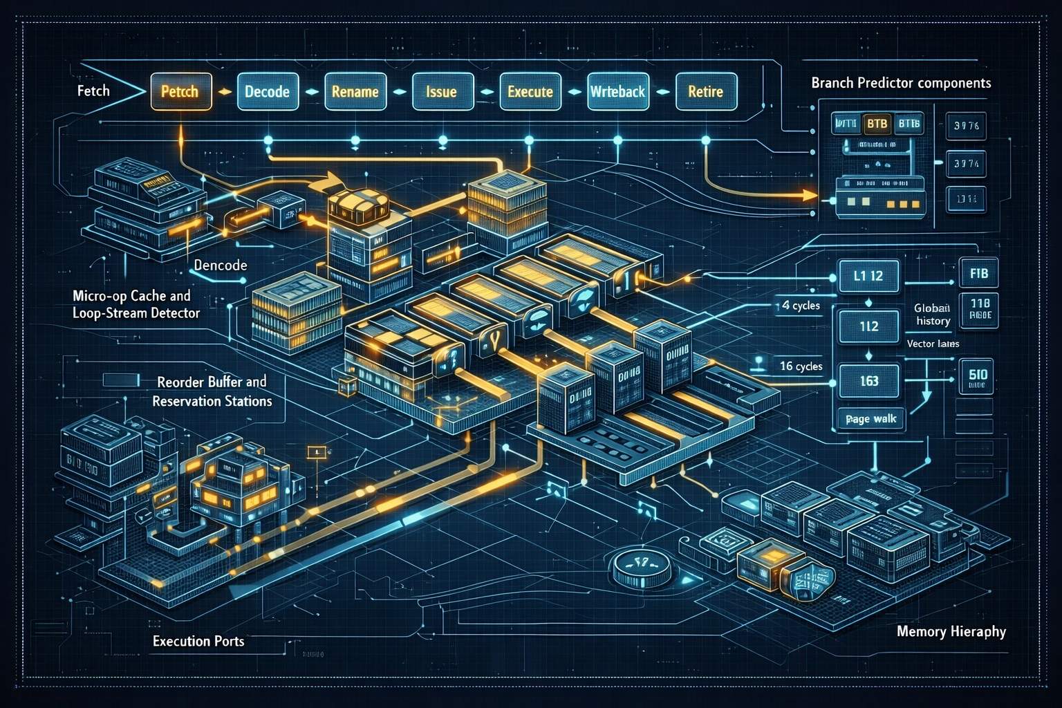
Hero image prompt (copy-ready): “Cutaway technical visualization of a CPU microarchitecture showing instruction fetch, decode, micro-op cache, rename & ROB, reservation stations, execution ports with ALU/FP/vector lanes, branch predictor structures (BTB, RSB, global history table), and memory hierarchy (L1/L2/L3/TLB) with latency numbers, schematic style, cyan & orange highlights, high-detail infographic, 3:2 aspect ratio, no logos or text overlays.”