Process Scheduling and Context Switching: How Operating Systems Share the CPU
A deep dive into how operating systems decide which process runs next and how they switch between processes. Understand scheduling algorithms, context switches, and the trade-offs that shape system responsiveness.
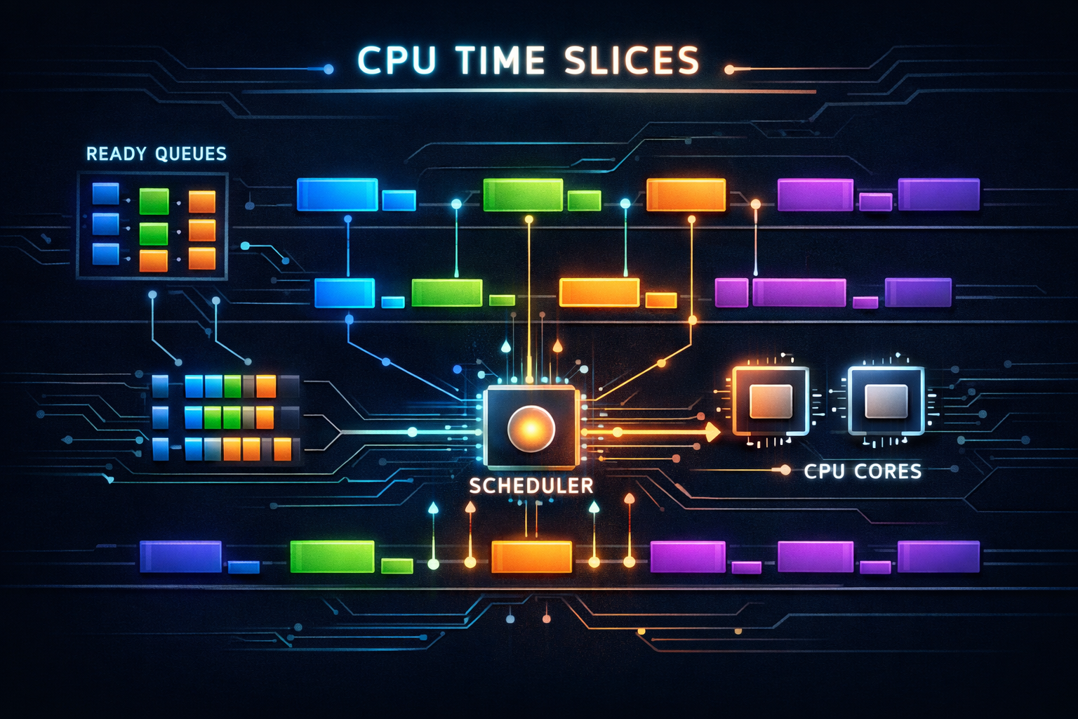
A single CPU core can only execute one instruction stream at a time, yet modern systems run hundreds of processes simultaneously. This illusion of parallelism requires the operating system to rapidly switch between processes, giving each a slice of CPU time. The scheduler—the component that decides who runs next—profoundly affects system responsiveness, throughput, and fairness. Understanding scheduling reveals why your interactive applications feel smooth or sluggish and why some workloads perform better than others.
1. The Scheduling Problem
Before diving into algorithms, let’s understand what the scheduler must accomplish.
1.1 Competing Goals
The scheduler must balance conflicting objectives:

Throughput:
- Maximize total work completed per unit time
- Minimize overhead (context switches, scheduling decisions)
- Keep CPU busy (high utilization)

Latency:
- Minimize response time for interactive tasks
- Reduce time from request to first response
- Quick reaction to user input

Fairness:
- Give each process reasonable share of CPU
- Prevent starvation (process never runs)
- Respect priorities without starving low-priority tasks

Energy efficiency:
- Allow CPU to enter low-power states
- Batch work to extend idle periods
- Balance performance with power consumption

These goals often conflict:
- High throughput wants fewer context switches
- Low latency wants more frequent switches
- Fairness may reduce throughput for high-priority tasks
1.2 Process States
Process lifecycle and state transitions:

          ┌─────────────────────────────────────────┐
          │                                         │
          ▼                                         │
     ┌─────────┐    schedule    ┌─────────────┐    │
     │  Ready  │───────────────►│   Running   │    │
     │         │◄───────────────│             │    │
     └─────────┘    preempt     └─────────────┘    │
          ▲                           │            │
          │                           │ wait       │
          │ I/O complete              ▼            │
          │                     ┌─────────────┐    │
          └─────────────────────│   Blocked   │    │
                                │  (Waiting)  │────┘
                                └─────────────┘
                                      │
                                      │ exit
                                      ▼
                                ┌─────────────┐
                                │  Terminated │
                                └─────────────┘

Ready: Waiting for CPU, can run immediately
Running: Currently executing on a CPU
Blocked: Waiting for I/O or event, cannot run
Terminated: Finished execution, awaiting cleanup
1.3 Types of Workloads
Different workloads have different needs:

CPU-bound (compute-intensive):
- Scientific computing, video encoding, compilation
- Want long time slices (minimize context switch overhead)
- Throughput is primary concern
- Example: Matrix multiplication

I/O-bound (interactive):
- Text editors, web browsers, terminals
- Frequently wait for I/O
- Want quick response when I/O completes
- Example: Waiting for keypress

Mixed:
- Most real applications
- Periods of computation interspersed with I/O
- Need adaptive scheduling
- Example: Web server processing requests

Real-time:
- Audio/video playback, industrial control
- Strict timing deadlines
- Missing deadline = failure
- Example: Audio buffer must refill every 5ms
2. Scheduling Algorithms
Different algorithms optimize for different goals.
2.1 First-Come, First-Served (FCFS)
Simplest possible scheduler:

Run processes in arrival order until they block or finish.

Arrival: P1(24ms), P2(3ms), P3(3ms)

Timeline:
├────────────────────────┼───┼───┤
│          P1            │P2 │P3 │
0                       24  27  30

Waiting times:
P1: 0ms
P2: 24ms
P3: 27ms
Average: 17ms

Problem: Convoy effect
Long process blocks short processes
Terrible for interactive workloads

If arrival order were P2, P3, P1:
├───┼───┼────────────────────────┤
│P2 │P3 │          P1            │
0   3   6                       30

Average wait: 3ms (much better!)
2.2 Shortest Job First (SJF)
Run shortest job next (optimal for minimizing average wait):

Same processes: P1(24ms), P2(3ms), P3(3ms)

SJF order:
├───┼───┼────────────────────────┤
│P2 │P3 │          P1            │
0   3   6                       30

Waiting times:
P2: 0ms
P3: 3ms
P1: 6ms
Average: 3ms (optimal!)

Problems:
1. Requires knowing job length in advance
   - Can estimate from history
   - Exponential averaging: τ(n+1) = α·t(n) + (1-α)·τ(n)

2. Starvation
   - Long jobs may never run if short jobs keep arriving
   - Need aging mechanism

3. Non-preemptive
   - Long job blocks everything once started
2.3 Round Robin
Each process gets a time quantum, then preempted:

Quantum = 4ms
Processes: P1(24ms), P2(3ms), P3(3ms)

Timeline:
├────┼───┼───┼────┼────┼────┼────┼────┼────┤
│ P1 │P2 │P3 │ P1 │ P1 │ P1 │ P1 │ P1 │ P1 │
0    4   7  10   14   18   22   26   30

Turnaround times:
P1: 30ms (vs 24ms in FCFS)
P2: 7ms  (vs 27ms in FCFS)
P3: 10ms (vs 30ms in FCFS)

Trade-off: Quantum size

Large quantum (100ms):
+ Less context switch overhead
- Approaches FCFS behavior
- Poor response time

Small quantum (1ms):
+ Better response time
+ Fairer distribution
- High context switch overhead
- Reduced throughput

Typical: 10-100ms depending on system type
2.4 Priority Scheduling
Each process has a priority, highest priority runs:

Priority levels (lower number = higher priority):
P1: priority 3, 10ms
P2: priority 1, 5ms
P3: priority 2, 2ms

Execution order:
├─────┼──┼──────────┤
│ P2  │P3│    P1    │
0     5  7         17

Problems:
1. Starvation of low-priority processes
   Solution: Aging - increase priority over time

2. Priority inversion
   High-priority task waits for low-priority task holding lock
   Solution: Priority inheritance

Priority inversion example:
High (H), Medium (M), Low (L)

L acquires lock
L preempted by M (M runs, doesn't need lock)
H becomes ready, needs lock
H blocked on L (who holds lock)
M keeps running (higher priority than L)
H effectively has lower priority than M!

Priority inheritance:
When H blocks on L's lock, L inherits H's priority
L runs, releases lock
H acquires lock and runs
2.5 Multilevel Feedback Queue
Combines multiple algorithms with adaptive behavior:

Queue 0 (highest priority): Round-robin, quantum = 8ms
Queue 1 (medium priority):  Round-robin, quantum = 16ms
Queue 2 (lowest priority):  FCFS

Rules:
1. New processes enter highest-priority queue
2. If process uses entire quantum, move to lower queue
3. If process blocks before quantum expires, stay in queue
4. Periodically boost all processes to top queue

Behavior:
- Interactive processes stay in high-priority queues
  (they block on I/O before using quantum)
- CPU-bound processes sink to lower queues
  (they use full quantum, get demoted)
- Prevents starvation through periodic boosting

┌───────────────────────────┐
│ Queue 0: ○ ○ ○            │ ← Interactive, short quantum
├───────────────────────────┤
│ Queue 1: ○ ○              │ ← Mixed workloads
├───────────────────────────┤
│ Queue 2: ○ ○ ○ ○ ○        │ ← CPU-bound, long/no quantum
└───────────────────────────┘
3. Modern Linux Scheduler: CFS
The Completely Fair Scheduler powers most Linux systems.
3.1 Virtual Runtime
CFS tracks "virtual runtime" (vruntime) for each task:

vruntime = actual runtime × (base priority / task priority)

Higher priority = vruntime increases slower
Lower priority = vruntime increases faster

Scheduler always picks task with lowest vruntime:

Tasks after some execution:
┌────────┬──────────┬──────────┐
│  Task  │ Priority │ vruntime │
├────────┼──────────┼──────────┤
│   A    │   120    │   50ms   │ ← Will run next
│   B    │   120    │   80ms   │
│   C    │   100    │   45ms   │ ← Higher priority
│   D    │   139    │   60ms   │ ← Lower priority
└────────┴──────────┴──────────┘

After C runs for 10ms (actual):
C's vruntime increase = 10ms × (120/100) = 12ms
C's new vruntime = 45 + 12 = 57ms

This naturally achieves weighted fair sharing:
- Higher-priority tasks get more CPU time
- All tasks make progress (no starvation)
3.2 Red-Black Tree Organization
CFS maintains runnable tasks in a red-black tree:

                    ┌───────────┐
                    │ vruntime  │
                    │    80     │
                    └─────┬─────┘
                   ╱             ╲
          ┌───────┴───┐       ┌───┴───────┐
          │ vruntime  │       │ vruntime  │
          │    50     │       │   100     │
          └─────┬─────┘       └───────────┘
               ╱ ╲
      ┌───────┴┐ ┌┴───────┐
      │   30   │ │   60   │
      └────────┘ └────────┘
           ↑
      Leftmost = next to run

Properties:
- O(log n) insertion and deletion
- O(1) access to leftmost (cached)
- Self-balancing maintains performance
- Efficiently handles thousands of tasks
3.3 Time Slice Calculation
CFS doesn't use fixed time slices:

Target latency: Maximum time before all tasks run once
- Default: 6ms for ≤8 tasks, 0.75ms per task beyond

Minimum granularity: Minimum time slice to avoid thrashing
- Default: 0.75ms

Time slice = target_latency × (task_weight / total_weight)

Example with 4 tasks:
Target latency = 6ms
All same priority (weight 1024 each)
Time slice = 6ms × (1024 / 4096) = 1.5ms each

With different priorities:
Task A: nice 0, weight 1024
Task B: nice 5, weight 335
Total weight = 1359

Task A slice = 6ms × (1024/1359) = 4.5ms
Task B slice = 6ms × (335/1359) = 1.5ms

Higher priority = larger time slice
3.4 Nice Values and Weights
Nice values range from -20 (highest priority) to +19 (lowest):

Nice value → Weight mapping (exponential):
┌──────┬────────┬─────────────────────────────┐
│ Nice │ Weight │ CPU share (vs nice 0)       │
├──────┼────────┼─────────────────────────────┤
│ -20  │  88761 │ 86.7× more than nice 0      │
│ -10  │   9548 │ 9.3× more than nice 0       │
│  -5  │   3121 │ 3.0× more than nice 0       │
│   0  │   1024 │ 1.0× (baseline)             │
│   5  │    335 │ 0.33× of nice 0             │
│  10  │    110 │ 0.11× of nice 0             │
│  19  │     15 │ 0.015× of nice 0            │
└──────┴────────┴─────────────────────────────┘

Each nice level ≈ 10% difference in CPU time
nice -1 vs nice 0 → ~10% more CPU
nice 1 vs nice 0 → ~10% less CPU
4. Real-Time Scheduling
For workloads with strict timing requirements.
4.1 Real-Time Priority Classes
Linux scheduling classes (highest to lowest priority):

1. SCHED_DEADLINE
   - Earliest Deadline First (EDF)
   - Task specifies runtime, deadline, period
   - Guaranteed to meet deadline if admitted

2. SCHED_FIFO
   - Real-time FIFO
   - Runs until blocks or higher priority arrives
   - No time slicing within priority level

3. SCHED_RR
   - Real-time Round Robin
   - Like FIFO but with time slicing
   - Same priority tasks share CPU

4. SCHED_OTHER (SCHED_NORMAL)
   - Default, CFS scheduler
   - Non-real-time tasks

5. SCHED_BATCH
   - For batch jobs, slightly disfavored
   - Won't preempt interactive tasks

6. SCHED_IDLE
   - Only runs when nothing else to do
   - For truly background work
4.2 Deadline Scheduling
SCHED_DEADLINE parameters:

Runtime:  How much CPU time needed per period
Deadline: Must complete within this time from start
Period:   How often task runs

Example: Audio processing
Period = 10ms (100 buffers/second)
Runtime = 2ms (computation needed)
Deadline = 10ms (must finish before next period)

Timeline:
├─────────┼─────────┼─────────┼─────────┤
│  2ms    │  idle   │  2ms    │  idle   │
├─────────┼─────────┼─────────┼─────────┤
│←  10ms period  →│←  10ms period  →│

Admission control:
System ensures Σ(runtime/period) ≤ 1.0
Otherwise deadlines cannot be guaranteed

Setting in Linux:
struct sched_attr attr = {
    .sched_policy = SCHED_DEADLINE,
    .sched_runtime = 2000000,   // 2ms in ns
    .sched_deadline = 10000000, // 10ms in ns
    .sched_period = 10000000,   // 10ms in ns
};
sched_setattr(0, &attr, 0);
4.3 Priority Inversion Solutions
Real-time systems must handle priority inversion:

Problem scenario:
1. Low-priority task L holds mutex M
2. High-priority task H arrives, needs M
3. H blocks waiting for L
4. Medium-priority task M arrives
5. M preempts L (M > L priority)
6. H effectively blocked by M (M doesn't need mutex!)

Priority Inheritance Protocol (PIP):
- When H blocks on mutex held by L
- L temporarily inherits H's priority
- L can't be preempted by M
- L releases mutex, drops to original priority
- H runs immediately

Priority Ceiling Protocol (PCP):
- Each mutex has ceiling = highest priority of users
- Task holding mutex runs at ceiling priority
- Prevents blocking by medium-priority tasks
- Also prevents deadlock

┌─────────────────────────────────────────────────┐
│ Without inheritance:     With inheritance:      │
│                                                 │
│ H: ██░░░░░░░░░░░░██      H: ██░░░░████          │
│ M: ░░░░░████████░░░      M: ░░░░░░░░████        │
│ L: ██████░░░░░░░░░░      L: ████████░░░░        │
│        ↑ M preempts L     ↑ L inherits H's pri │
└─────────────────────────────────────────────────┘
5. Context Switching
The mechanics of switching between processes.
5.1 What Must Be Saved
Context switch saves and restores process state:

CPU Registers:
┌────────────────────────────────────────────────┐
│ General purpose: RAX, RBX, RCX, RDX, RSI, RDI  │
│                  R8-R15, RBP, RSP              │
│ Instruction pointer: RIP                        │
│ Flags: RFLAGS                                  │
│ Segment registers: CS, DS, ES, FS, GS, SS     │
│ Control registers: CR3 (page table base)       │
│ FPU/SIMD: x87 state, XMM0-15, YMM, ZMM        │
└────────────────────────────────────────────────┘

Kernel stack:
- Each process has kernel stack
- Contains syscall frames, interrupt handlers

Memory management:
- CR3 register points to page table
- TLB may need flushing (or use ASID/PCID)

Other state:
- File descriptors (not saved per switch)
- Signal handlers
- Thread-local storage pointer
5.2 Context Switch Overhead
Direct costs:
1. Save old process registers (~100 cycles)
2. Load new process registers (~100 cycles)
3. Switch page tables (modify CR3)
4. Scheduler decision logic
Total direct: ~1000-5000 cycles

Indirect costs (often larger):
1. TLB flush
   - All translations invalid
   - Page table walks on every access
   - 100s of cycles per miss until warm

2. Cache pollution
   - New process has different working set
   - Cache misses until data loaded
   - Can be millions of cycles

3. Pipeline flush
   - CPU pipeline cleared
   - Branch predictor useless for new code

Measurements:
- Minimal switch: 1-5 microseconds
- With TLB miss penalties: 10-100 microseconds
- With cache misses: 100s of microseconds
5.3 Hardware Context Switch Support
x86 TSS (Task State Segment):
- Hardware-supported context switch
- Single instruction: JMP to TSS
- Rarely used in modern OS (too inflexible, slow)

Modern approach: Software context switch

// Simplified Linux context switch (x86-64)
switch_to(prev, next):
    // Save callee-saved registers on kernel stack
    push rbp
    push rbx
    push r12
    push r13
    push r14
    push r15

    // Switch kernel stacks
    mov [prev->thread.sp], rsp
    mov rsp, [next->thread.sp]

    // Switch page tables
    mov cr3, [next->mm.pgd]

    // Restore callee-saved registers
    pop r15
    pop r14
    pop r13
    pop r12
    pop rbx
    pop rbp

    // Return to new process (RIP on stack)
    ret
5.4 Reducing Context Switch Cost
TLB management:
- PCID (Process Context ID): Tag TLB entries
  - No flush needed, entries distinguished by ID
  - Limited IDs (4096 on x86)
  - Huge performance improvement

- ASID (Address Space ID): ARM equivalent
  - 8 or 16 bits depending on implementation

Lazy FPU switching:
- Don't save/restore FPU state immediately
- Mark FPU as "not owned" by new process
- Only save/restore on first FPU instruction
- Many processes never use FPU

Batching scheduler work:
- Amortize scheduling overhead
- Don't switch for very short time slices
- Minimum granularity prevents thrashing
6. Multiprocessor Scheduling
Scheduling across multiple CPUs adds complexity.
6.1 SMP Scheduling Challenges
Symmetric Multiprocessing (SMP) issues:

1. Load balancing
   All CPUs should be equally utilized
   Idle CPU should steal work from busy CPU

   CPU 0: [████████]  CPU 1: [██░░░░░░]
          ↑ Overloaded        ↑ Underutilized

2. Cache affinity
   Process benefits from running on same CPU
   Cache contents remain relevant
   Moving process = cold cache

3. Lock contention
   Scheduler data structures need synchronization
   Single run queue = bottleneck

4. NUMA awareness
   Prefer running near process's memory
   Cross-socket migration is expensive
6.2 Per-CPU Run Queues
Modern Linux: Each CPU has its own run queue

┌─────────────────┐  ┌─────────────────┐
│     CPU 0       │  │     CPU 1       │
│ ┌─────────────┐ │  │ ┌─────────────┐ │
│ │  Run Queue  │ │  │ │  Run Queue  │ │
│ │ ○ ○ ○ ○     │ │  │ │ ○ ○         │ │
│ └─────────────┘ │  │ └─────────────┘ │
│ ┌─────────────┐ │  │ ┌─────────────┐ │
│ │  Running: A │ │  │ │  Running: B │ │
│ └─────────────┘ │  │ └─────────────┘ │
└─────────────────┘  └─────────────────┘

Benefits:
- No lock contention for scheduling decisions
- Each CPU schedules independently
- Cache-hot data stays on same CPU

Challenges:
- Must balance load across queues
- Migration decisions need care
6.3 Load Balancing
Linux load balancing hierarchy:

Scheduling domains:
┌───────────────────────────────────────────────────┐
│                  System Domain                     │
│  ┌────────────────────┐  ┌────────────────────┐   │
│  │    NUMA Node 0     │  │    NUMA Node 1     │   │
│  │  ┌──────┐ ┌──────┐ │  │  ┌──────┐ ┌──────┐ │   │
│  │  │CPU 0 │ │CPU 1 │ │  │  │CPU 2 │ │CPU 3 │ │   │
│  │  │ SMT  │ │ SMT  │ │  │  │ SMT  │ │ SMT  │ │   │
│  │  │ pair │ │ pair │ │  │  │ pair │ │ pair │ │   │
│  │  └──────┘ └──────┘ │  │  └──────┘ └──────┘ │   │
│  └────────────────────┘  └────────────────────┘   │
└───────────────────────────────────────────────────┘

Balancing frequency:
- Within SMT pair: Most frequent
- Within NUMA node: Frequent
- Across NUMA nodes: Least frequent (expensive)

Balance triggers:
- Periodic timer (every few ms)
- CPU goes idle (work stealing)
- Fork/exec (spread new work)
6.4 Cache Affinity
Scheduling considers CPU affinity:

Soft affinity (default):
- Prefer same CPU but migrate if needed
- Scheduler tracks last CPU ran on
- Migration only if imbalance significant

Hard affinity (sched_setaffinity):
- Process restricted to specific CPUs
- Used for NUMA optimization
- Used for isolating real-time tasks

CPU affinity mask:
0b1111  = CPUs 0,1,2,3
0b0011  = CPUs 0,1 only
0b1000  = CPU 3 only

// Set affinity in C
cpu_set_t mask;
CPU_ZERO(&mask);
CPU_SET(0, &mask);  // CPU 0 only
sched_setaffinity(0, sizeof(mask), &mask);

// Command line
taskset -c 0,1 ./myprogram  // Run on CPUs 0 and 1
7. Thread Scheduling
Threads within a process share address space.
7.1 User vs Kernel Threads
Kernel threads (1:1 model):
- Each user thread = one kernel thread
- OS schedules directly
- Can utilize multiple CPUs
- Used by Linux, Windows, macOS

User threads (N:1 model):
- Many user threads = one kernel thread
- User-space scheduler (runtime library)
- Cannot use multiple CPUs
- Fast switching (no syscall)
- If one blocks, all block
- Historical model, rarely used now

Hybrid (M:N model):
- M user threads on N kernel threads
- User-space + kernel scheduling
- Complex to implement correctly
- Used by Go, some historical systems

┌─────────────────────────────────────────────────┐
│                   1:1 Model                      │
│  User:   [T1] [T2] [T3] [T4]                    │
│            │    │    │    │                     │
│  Kernel: [K1] [K2] [K3] [K4]                    │
│                                                 │
│                   M:N Model                      │
│  User:   [T1] [T2] [T3] [T4] [T5] [T6]         │
│            ╲   │   ╱     ╲   │   ╱              │
│  Kernel:   [K1]  [K2]    [K3]                   │
└─────────────────────────────────────────────────┘
7.2 Go’s Goroutine Scheduler
Go runtime: M:N scheduling with work stealing

Components:
G = Goroutine (user thread)
M = Machine (OS thread)
P = Processor (logical CPU, runs G's)

Structure:
┌─────────────────────────────────────────────────┐
│                 Go Runtime                       │
│                                                 │
│  ┌─────┐ ┌─────┐         Global Queue           │
│  │  P  │ │  P  │         [G] [G] [G]            │
│  │     │ │     │                                │
│  │Local│ │Local│                                │
│  │Queue│ │Queue│                                │
│  │[G G]│ │[G G]│                                │
│  │     │ │     │                                │
│  │  M ─┼─┼─ M  │   M (spare, waiting for P)     │
│  └──│──┘ └──│──┘                                │
│     │       │                                   │
│  ───┴───────┴─── OS Scheduler                   │
└─────────────────────────────────────────────────┘

Work stealing:
1. P runs goroutines from local queue
2. Local queue empty? Steal from another P
3. No work anywhere? Check global queue
4. Still nothing? Poll network
5. Finally: Put M to sleep

Benefits:
- Millions of goroutines possible
- Fast context switch (~200ns vs ~1μs for threads)
- Automatic load balancing
7.3 Cooperative vs Preemptive
Cooperative scheduling:
- Task explicitly yields control
- No involuntary preemption
- Risk: Misbehaving task hogs CPU

// Cooperative example (Go pre-1.14)
for i := 0; i < 1e9; i++ {
    compute()  // No function calls = no preemption point
}
// Other goroutines starved!

Preemptive scheduling:
- Timer interrupts force yield
- OS/runtime can preempt any time
- More complex but fairer

Go 1.14+ async preemption:
- Signal-based preemption
- Inject preemption at safepoints
- Loops without calls can still be preempted

Linux PREEMPT configurations:
PREEMPT_NONE:     Server workloads, higher throughput
PREEMPT_VOLUNTARY: Desktop, balance throughput/latency
PREEMPT:          Low-latency desktop/audio
PREEMPT_RT:       Real-time, minimal latency
8. Scheduling in Practice
Real-world considerations and tools.
8.1 Examining Scheduler Behavior
# View process scheduling info
ps -eo pid,ni,pri,cls,psr,comm
# ni: nice value, pri: priority, cls: class, psr: CPU

# Real-time attributes
chrt -p PID

# Set scheduling policy
chrt -f -p 50 PID    # SCHED_FIFO, priority 50
chrt -r -p 50 PID    # SCHED_RR, priority 50
chrt -o -p 0 PID     # SCHED_OTHER

# Change nice value
nice -n 10 ./myprogram    # Start with nice 10
renice -n 5 -p PID        # Change running process

# CPU affinity
taskset -p PID            # Show affinity
taskset -cp 0,1 PID       # Set to CPUs 0 and 1

# Detailed scheduler statistics
cat /proc/PID/sched
8.2 Scheduler Tracing
# Trace context switches
perf sched record ./myprogram
perf sched latency    # Scheduling latency stats
perf sched map        # Visual CPU timeline
perf sched timehist   # Detailed timing history

# Example output from perf sched latency:
 Task                  | Runtime   | Switches | Avg delay |
 myprogram (12345)     | 500.000ms |     2000 |    0.050ms|
 kworker/0:1 (123)     |  10.000ms |       50 |    0.100ms|

# ftrace for detailed analysis
echo 1 > /sys/kernel/debug/tracing/events/sched/enable
cat /sys/kernel/debug/tracing/trace_pipe

# Output shows every schedule event:
# <idle>-0 [000] 1234.567: sched_switch: prev=swapper next=myprogram
8.3 Scheduling Latency Measurement
// Measure scheduling latency
#include <time.h>
#include <sched.h>

void measure_latency() {
    struct timespec before, after;

    for (int i = 0; i < 10000; i++) {
        clock_gettime(CLOCK_MONOTONIC, &before);
        sched_yield();  // Voluntarily give up CPU
        clock_gettime(CLOCK_MONOTONIC, &after);

        long latency_ns = (after.tv_sec - before.tv_sec) * 1e9 +
                          (after.tv_nsec - before.tv_nsec);
        record_latency(latency_ns);
    }

    print_histogram();
}

// Typical results (microseconds):
// PREEMPT_NONE:  Median 5μs,  P99 100μs, P99.9 500μs
// PREEMPT:       Median 3μs,  P99 50μs,  P99.9 200μs
// PREEMPT_RT:    Median 2μs,  P99 10μs,  P99.9 50μs
8.4 Common Scheduling Issues
Problem: High scheduling latency
Symptoms:
- Application stutters
- Audio/video glitches
- Mouse lag

Diagnosis:
- perf sched latency shows high delays
- Check for CPU-bound processes
- Check for runaway interrupt handlers

Solutions:
- Increase priority (nice -20 or real-time)
- CPU affinity to isolate from other work
- Use PREEMPT kernel
- Check for lock contention

Problem: CPU imbalance
Symptoms:
- Some CPUs 100%, others idle
- Lower throughput than expected

Diagnosis:
- mpstat -P ALL 1 shows uneven usage
- Check affinity settings

Solutions:
- Remove unnecessary affinity constraints
- Check NUMA configuration
- Verify load balancing enabled

Problem: Priority inversion
Symptoms:
- High-priority task unexpectedly delayed
- Occurs around lock acquisition

Diagnosis:
- Trace shows high-pri blocked on low-pri
- Lock held during preemption

Solutions:
- Enable priority inheritance on mutexes
- Use lock-free algorithms
- Reduce critical section length
9. Scheduling for Specific Workloads
Tuning for different application types.
9.1 Interactive Desktop
Goals:
- Responsive UI (<100ms to user action)
- Smooth video/animation (16ms frames)
- Background tasks shouldn't interfere

Tuning:
- Use PREEMPT kernel
- Smaller scheduling granularity
- Boost priority of interactive tasks

systemd automatic boosting:
- Detects interactive processes
- Temporarily boosts on activity
- Drops priority when idle

cgroups for isolation:
# Limit background CPU
cgcreate -g cpu:background
echo 50000 > /sys/fs/cgroup/cpu/background/cpu.cfs_quota_us
# 50ms per 100ms = 50% max CPU for background group
9.2 Server Throughput
Goals:
- Maximum requests/second
- Efficient CPU utilization
- Minimize context switches

Tuning:
- PREEMPT_NONE or PREEMPT_VOLUNTARY kernel
- Larger time slices
- Affinity for connection handling

NUMA-aware server:
- Pin network queues to CPUs
- Keep connection state near handling CPU
- Avoid cross-NUMA migrations

irqbalance for interrupt distribution:
- Spread hardware interrupts across CPUs
- Match network IRQs to application threads

# Pin IRQ to specific CPU
echo 2 > /proc/irq/123/smp_affinity  # CPU 1
9.3 Real-Time Audio/Video
Goals:
- Never miss deadline (buffer underrun = glitch)
- Consistent latency
- Predictable timing

Tuning:
- PREEMPT_RT kernel
- SCHED_FIFO or SCHED_DEADLINE
- Memory locking (mlockall)
- CPU isolation (isolcpus)

Audio example (JACK):
# Run audio server with real-time priority
jackd -R -P 70 -d alsa -p 128 -n 2

Configuration:
- Buffer size: 128 samples
- Sample rate: 48000 Hz
- Latency: 128/48000 = 2.67ms per buffer
- Need to refill every 2.67ms!

CPU isolation:
# Boot parameter
isolcpus=2,3

# Run audio on isolated CPUs
taskset -c 2,3 jackd ...
# CPUs 2,3 run only audio, no interference
9.4 High-Performance Computing
Goals:
- Maximum FLOPS
- Efficient parallelization
- Predictable scaling

Tuning:
- Pin threads to CPUs (1:1 binding)
- Disable hyperthreading for some workloads
- NUMA-aware memory allocation

MPI process placement:
# OpenMPI binding
mpirun --bind-to core --map-by socket -np 64 ./simulation

# Process 0 on CPU 0, Process 1 on CPU 1, etc.
# Maximizes cache utilization
# Minimizes cross-socket communication

OpenMP thread affinity:
export OMP_PROC_BIND=close
export OMP_PLACES=cores
# Threads bound to adjacent cores

NUMA-aware allocation:
numactl --localalloc ./hpc_app
# Allocate memory on same node as running CPU
10. Future Directions
Emerging trends in scheduling.
10.1 Heterogeneous Computing
big.LITTLE / Intel Hybrid architecture:

Performance cores (P-cores): Fast, power-hungry
Efficient cores (E-cores): Slower, power-efficient

┌───────────────────────────────────────────────┐
│  P-core  │  P-core  │  E-core  │  E-core     │
│   Fast   │   Fast   │  Slow    │  Slow       │
│ 5.0 GHz  │ 5.0 GHz  │ 3.0 GHz  │ 3.0 GHz    │
└───────────────────────────────────────────────┘

Scheduling challenges:
- Which tasks go to which cores?
- How to measure task requirements?
- When to migrate between core types?

Intel Thread Director:
- Hardware hints about thread characteristics
- Guides OS scheduler decisions
- Learns from thread behavior

ARM DynamIQ:
- Similar hybrid approach
- Common in mobile devices
- Power efficiency critical
10.2 Energy-Aware Scheduling
Modern schedulers consider power:

DVFS (Dynamic Voltage and Frequency Scaling):
- Reduce frequency when load is light
- Lower voltage saves power quadratically
- Balance performance vs power

schedutil governor:
- Integrated with CFS scheduler
- Frequency scales with utilization
- Faster response than polling-based governors

Power-aware placement:
- Consolidate work on fewer cores
- Allow other cores to deep sleep
- Race-to-idle strategy

┌─────────────────────────────────────────────────┐
│ Traditional:       │ Power-aware:               │
│ CPU0: [███░░░░░]  │ CPU0: [████████]           │
│ CPU1: [███░░░░░]  │ CPU1: [sleeping]           │
│ CPU2: [███░░░░░]  │ CPU2: [sleeping]           │
│ CPU3: [███░░░░░]  │ CPU3: [sleeping]           │
│ All cores active   │ One core, three sleeping   │
└─────────────────────────────────────────────────┘
10.3 Machine Learning for Scheduling
Learned scheduling policies:

Traditional: Hand-tuned heuristics
ML approach: Learn from workload patterns

Google's Borg (cluster scheduling):
- ML predicts resource requirements
- Better bin packing
- Reduced resource waste

Research directions:
- Reinforcement learning for time slice selection
- Predicting process behavior from history
- Automatic parameter tuning

Challenges:
- Scheduling decisions must be fast (<1μs)
- ML inference overhead must be minimal
- Generalization across workloads
- Explainability for debugging
10.4 Microsecond-Scale Computing
Emerging workloads need μs scheduling:

FaaS (Functions as a Service):
- Function executes in <1ms
- Context switch overhead significant
- Startup latency critical

Storage (NVMe, Optane):
- Device latency <10μs
- Can't afford 10μs context switch
- Need kernel bypass or polling

DPDK/SPDK approach:
- User-space polling
- No context switches
- Dedicated cores
- Trade CPU for latency

io_uring approach:
- Asynchronous I/O
- Batch submissions
- Reduce syscall overhead
- Polling mode for lowest latency
11. Summary and Key Takeaways
Consolidating what we’ve learned about scheduling.
11.1 Core Concepts
Scheduling fundamentals:
✓ Scheduler decides which process runs when
✓ Balances throughput, latency, fairness, power
✓ Context switch saves/restores process state

Key algorithms:
✓ FCFS: Simple but convoy effect
✓ Round Robin: Fair but overhead
✓ Priority: Flexible but starvation risk
✓ CFS: Weighted fairness via virtual runtime

Context switch costs:
✓ Direct: Register save/restore (~1000 cycles)
✓ Indirect: TLB flush, cache pollution (>>direct)
✓ PCID/ASID reduces TLB flush cost

Multiprocessor:
✓ Per-CPU run queues avoid lock contention
✓ Load balancing keeps CPUs utilized
✓ Cache affinity vs load balance trade-off
11.2 Practical Guidelines
For application developers:

1. Understand your workload type
   - CPU-bound: Long slices, high priority
   - I/O-bound: Default scheduling usually fine
   - Real-time: Use SCHED_DEADLINE or SCHED_FIFO

2. Use appropriate APIs
   - nice/renice for simple priority
   - sched_setscheduler for scheduling class
   - sched_setaffinity for CPU pinning

3. Minimize unnecessary context switches
   - Batch work appropriately
   - Use async I/O when possible
   - Pool threads instead of constant creation

4. Profile before optimizing
   - perf sched shows actual behavior
   - Don't guess, measure

For system administrators:

1. Choose right kernel preemption level
   - Servers: PREEMPT_NONE or VOLUNTARY
   - Desktops: PREEMPT
   - Real-time: PREEMPT_RT

2. Configure cgroups for workload isolation
   - Limit background task CPU
   - Protect critical services

3. NUMA considerations
   - Monitor cross-node traffic
   - Pin important processes appropriately
11.3 Debugging Checklist
When investigating scheduling issues:

□ Check process priorities (ps -eo pid,ni,pri)
□ Examine CPU utilization per core (mpstat -P ALL)
□ Look for scheduling latency (perf sched latency)
□ Check for CPU affinity constraints (taskset)
□ Review cgroup limits
□ Examine context switch rates (vmstat)
□ Check for priority inversion (trace lock waits)
□ Verify NUMA placement (numastat)
□ Review kernel preemption configuration
□ Check for interrupt storms (watch /proc/interrupts)
The scheduler sits at the heart of every operating system, making thousands of decisions per second that determine how responsive your system feels and how efficiently it uses hardware resources. From the elegant simplicity of round-robin to the sophisticated fairness of CFS, from single-CPU time sharing to complex NUMA-aware load balancing, scheduling represents decades of research and engineering refinement. Understanding these mechanisms empowers you to tune systems for specific workloads, diagnose performance problems, and appreciate the invisible yet essential work that makes multitasking possible. Whether you’re building real-time systems, optimizing server throughput, or simply curious why your desktop feels smooth, the scheduler’s decisions shape every interaction you have with a computer. The interplay between hardware capabilities, operating system policies, and application requirements creates a rich design space where small changes can yield significant improvements in both performance and user experience.