TCP Congestion Control: From Slow Start to BBR
A comprehensive exploration of TCP congestion control algorithms, from classic approaches like Tahoe and Reno to modern innovations like BBR. Learn how these algorithms balance throughput, fairness, and latency across diverse network conditions.
Every time you load a webpage, stream a video, or download a file, TCP congestion control algorithms work invisibly to maximize throughput while preventing network collapse. These algorithms represent decades of research into one of networking’s hardest problems: how do independent senders share a network fairly without overwhelming it? Let’s explore how TCP congestion control evolved from simple beginnings to sophisticated model-based approaches.
1. The Congestion Problem
Without congestion control, networks collapse under load.
1.1 The Tragedy of the Commons
Consider multiple TCP senders sharing a bottleneck link:
Sender A ──┐
           │
Sender B ──┼──[ Bottleneck: 100 Mbps ]──→ Receiver
           │
Sender C ──┘

If each sender transmits at 50 Mbps:
Total offered load: 150 Mbps
Bottleneck capacity: 100 Mbps
Result: Packet loss, retransmissions, collapse
Without coordination, each sender’s rational behavior (send as fast as possible) leads to collective disaster.
1.2 Congestion Collapse
The 1986 Internet congestion collapse demonstrated this dramatically:
Before collapse:
- Network throughput: ~32 Kbps
- Offered load increasing

During collapse:
- Offered load: >> capacity
- Actual throughput: dropped to ~100 bps
- 99.7% of bandwidth wasted on retransmissions!
Packets were being retransmitted multiple times, each retransmission adding to congestion, causing more loss, causing more retransmissions—a death spiral.
1.3 The Solution: Congestion Control
Van Jacobson’s 1988 algorithms saved the Internet:
Key insight: Use packet loss as a signal of congestion

Core mechanisms:
1. Slow start: Probe for available bandwidth
2. Congestion avoidance: Gentle increase after finding capacity
3. Fast retransmit: Quickly detect and recover from loss
4. Fast recovery: Maintain throughput during recovery
2. TCP Fundamentals
Before diving into algorithms, let’s establish key concepts.
2.1 The Congestion Window
The congestion window (cwnd) limits how much data can be in flight:
# Simplified TCP sender logic
def send_data(self):
    while True:
        # Can only send if within both windows
        bytes_in_flight = self.sent_but_unacked

        send_window = min(self.cwnd, self.receiver_window)
        available = send_window - bytes_in_flight

        if available > 0:
            self.send_segment(min(available, MSS))
cwnd controls sending rate:
- Small cwnd → slow sending → low throughput
- Large cwnd → fast sending → high throughput (until loss)

Effective rate ≈ cwnd / RTT
2.2 Round-Trip Time (RTT)
RTT is the time for a packet to reach the receiver and for its acknowledgment to return:
Sender                                    Receiver
  │                                          │
  │────────── Data packet ─────────────────→│
  │                                          │
  │←──────────── ACK ────────────────────────│
  │                                          │
  │◄─────────────── RTT ───────────────────►│
RTT affects everything:
- Throughput:
max_rate = cwnd / RTT - Responsiveness: How quickly we detect congestion
- Fairness: Flows with different RTTs compete unequally
2.3 Bandwidth-Delay Product
The BDP is the amount of data “in flight” to fully utilize a link:
BDP = Bandwidth × RTT

Example:
- 1 Gbps link
- 50 ms RTT
- BDP = 1,000,000,000 bits/s × 0.050 s = 50,000,000 bits = 6.25 MB

To fully utilize this link, cwnd must reach 6.25 MB!
This is why high-bandwidth, high-latency networks (like satellite links or transcontinental connections) are challenging.
2.4 Loss Detection
TCP detects loss through two mechanisms:
# Timeout-based detection
if time_since_send > RTO:
    # RTO = Retransmission Timeout (estimated from RTT)
    handle_timeout_loss()

# Duplicate ACK detection
if duplicate_acks >= 3:
    # Receiver got out-of-order packets
    # Indicates a gap (lost packet)
    handle_fast_retransmit()
Three duplicate ACKs trigger fast retransmit, avoiding the long RTO wait.
3. Classic Congestion Control
The original algorithms that saved the Internet.
3.1 Slow Start
Despite the name, slow start grows exponentially:
def slow_start(self, ack_received):
    # Double cwnd every RTT
    self.cwnd += MSS  # Called for each ACK

    # With each ACK acknowledging MSS bytes,
    # and each RTT seeing cwnd/MSS ACKs,
    # cwnd doubles each RTT
RTT 0: cwnd = 1 MSS    (1 segment in flight)
RTT 1: cwnd = 2 MSS    (2 segments)
RTT 2: cwnd = 4 MSS    (4 segments)
RTT 3: cwnd = 8 MSS    (8 segments)
...
Exponential growth until loss or ssthresh
Slow start ends when:
- cwnd reaches slow start threshold (ssthresh)
- Packet loss is detected
3.2 Congestion Avoidance
After slow start, growth becomes linear:
def congestion_avoidance(self, ack_received):
    # Increase cwnd by 1 MSS per RTT
    self.cwnd += MSS * (MSS / self.cwnd)

    # Alternative: count ACKs
    # self.cwnd_count += 1
    # if self.cwnd_count >= self.cwnd / MSS:
    #     self.cwnd += MSS
    #     self.cwnd_count = 0
Linear growth: cwnd increases by 1 MSS per RTT

RTT 10: cwnd = 20 MSS
RTT 11: cwnd = 21 MSS
RTT 12: cwnd = 22 MSS
...
Gentle probing for more bandwidth
3.3 TCP Tahoe
The first complete congestion control algorithm (1988):
class TCPTahoe:
    def __init__(self):
        self.cwnd = MSS
        self.ssthresh = float('inf')

    def on_ack(self):
        if self.cwnd < self.ssthresh:
            # Slow start
            self.cwnd += MSS
        else:
            # Congestion avoidance
            self.cwnd += MSS * MSS / self.cwnd

    def on_loss(self):
        # Any loss: reset to slow start
        self.ssthresh = self.cwnd / 2
        self.cwnd = MSS
        # Retransmit from slow start
Tahoe behavior (sawtooth pattern):

cwnd
  ▲
  │     ╱╲
  │    ╱  ╲
  │   ╱    ╲
  │  ╱      ╲      ╱╲
  │ ╱        ╲    ╱  ╲
  │╱          ╲  ╱    ╲
  └────────────────────────→ time
       loss    loss
Tahoe’s weakness: complete reset on any loss is expensive.
3.4 TCP Reno
Reno (1990) added fast recovery:
class TCPReno:
    def __init__(self):
        self.cwnd = MSS
        self.ssthresh = float('inf')
        self.dup_acks = 0

    def on_ack(self):
        if self.in_fast_recovery:
            # Exit fast recovery
            self.cwnd = self.ssthresh
            self.in_fast_recovery = False
        elif self.cwnd < self.ssthresh:
            self.cwnd += MSS  # Slow start
        else:
            self.cwnd += MSS * MSS / self.cwnd  # Congestion avoidance
        self.dup_acks = 0

    def on_dup_ack(self):
        self.dup_acks += 1
        if self.dup_acks == 3:
            # Fast retransmit
            self.ssthresh = self.cwnd / 2
            self.cwnd = self.ssthresh + 3 * MSS
            self.in_fast_recovery = True
            self.retransmit_lost_segment()
        elif self.in_fast_recovery:
            # Inflate cwnd for each dup ACK
            self.cwnd += MSS

    def on_timeout(self):
        # Timeout: back to slow start
        self.ssthresh = self.cwnd / 2
        self.cwnd = MSS
        self.in_fast_recovery = False
Fast recovery allows Reno to maintain half its rate after loss instead of resetting completely.
3.5 TCP NewReno
NewReno (1999) handles multiple losses in one window:
class TCPNewReno(TCPReno):
    def __init__(self):
        super().__init__()
        self.recover_seq = 0

    def on_dup_ack(self):
        self.dup_acks += 1
        if self.dup_acks == 3 and not self.in_fast_recovery:
            # Enter fast recovery
            self.ssthresh = self.cwnd / 2
            self.cwnd = self.ssthresh + 3 * MSS
            self.in_fast_recovery = True
            self.recover_seq = self.highest_sent_seq
            self.retransmit_lost_segment()
        elif self.in_fast_recovery:
            self.cwnd += MSS

    def on_ack(self, ack_seq):
        if self.in_fast_recovery:
            if ack_seq >= self.recover_seq:
                # Full recovery: all lost packets retransmitted
                self.cwnd = self.ssthresh
                self.in_fast_recovery = False
            else:
                # Partial ACK: more packets were lost
                self.retransmit_next_segment()
                self.cwnd -= (ack_seq - self.last_ack)  # Deflate
                self.cwnd += MSS  # Re-inflate by 1
        else:
            # Normal operation
            super().on_ack()
NewReno stays in fast recovery until all losses from a single congestion event are recovered.
4. Loss-Based Algorithms
Modern loss-based algorithms improve on Reno’s foundations.
4.1 TCP CUBIC
CUBIC (2008) is the default algorithm in Linux:
class TCPCUBIC:
    def __init__(self):
        self.cwnd = MSS
        self.w_max = 0  # cwnd at last loss
        self.k = 0      # Time to reach w_max
        self.t = 0      # Time since last loss
        self.C = 0.4    # CUBIC constant
        self.beta = 0.7 # Multiplicative decrease factor

    def on_ack(self):
        self.t = time_since_last_loss()

        # CUBIC function: W(t) = C(t-K)³ + W_max
        self.k = (self.w_max * (1 - self.beta) / self.C) ** (1/3)
        w_cubic = self.C * (self.t - self.k) ** 3 + self.w_max

        # Also compute TCP-friendly rate
        w_tcp = self.w_max * self.beta + 3 * (1 - self.beta) / (1 + self.beta) * self.t / self.rtt

        # Use the larger of CUBIC and TCP-friendly
        self.cwnd = max(w_cubic, w_tcp)

    def on_loss(self):
        self.w_max = self.cwnd
        self.cwnd = self.cwnd * self.beta
        self.t = 0
CUBIC’s key insight: use a cubic function to probe for bandwidth:
CUBIC cwnd over time:

cwnd
  ▲
  │         w_max ──────────────────────
  │        ╱    ╲
  │       ╱      ╲
  │      ╱        ╲     probe above
  │     ╱          ╲    w_max
  │────╱────────────╲───────────────────
  │   ╱ plateau      ╲
  │  ╱                 aggressive
  │ ╱ aggressive        recovery
  │╱  recovery
  └────────────────────────────────────→ time
      loss          loss
- Aggressive recovery: Quick ramp back to previous rate
- Plateau near W_max: Gentle probing
- Above W_max: Explore for more bandwidth
4.2 TCP PRR (Proportional Rate Reduction)
PRR (2013) improves loss recovery:
def proportional_rate_reduction(self, in_flight, ssthresh, ack_delivered):
    """
    RFC 6937: Reduce cwnd proportionally to loss,
    spreading retransmissions across the recovery period.
    """
    if in_flight > ssthresh:
        # PRR-SSRB: slow reduction
        sndcnt = max(ack_delivered * ssthresh / recovery_cwnd, 1)
    else:
        # PRR-CRB: catch up
        sndcnt = max(ack_delivered, 1)

    return sndcnt
PRR spreads retransmissions evenly rather than bursting, reducing buffer pressure.
4.3 HTCP (Hamilton TCP)
HTCP adapts aggressiveness based on RTT:
class HTCP:
    def __init__(self):
        self.alpha = 1
        self.beta = 0.5
        self.delta = 0  # Time since last loss

    def compute_alpha(self):
        """Increase aggressiveness over time."""
        if self.delta < 1:
            return 1
        else:
            # More aggressive as time since loss grows
            return 1 + 10 * (self.delta - 1) + 0.5 * (self.delta - 1) ** 2

    def on_ack(self):
        self.alpha = self.compute_alpha()
        self.cwnd += self.alpha / self.cwnd
HTCP is more aggressive on long-RTT paths, improving fairness between flows.
5. Delay-Based Algorithms
Loss-based algorithms fill buffers before detecting congestion. Delay-based algorithms use RTT increase as an earlier signal.
5.1 TCP Vegas
Vegas (1995) pioneered delay-based congestion control:
class TCPVegas:
    def __init__(self):
        self.cwnd = MSS
        self.base_rtt = float('inf')  # Minimum observed RTT
        self.alpha = 2  # Lower threshold
        self.beta = 4   # Upper threshold

    def on_ack(self, rtt):
        self.base_rtt = min(self.base_rtt, rtt)

        # Expected rate if no queuing
        expected = self.cwnd / self.base_rtt

        # Actual rate with current RTT
        actual = self.cwnd / rtt

        # Difference is queued data
        diff = (expected - actual) * self.base_rtt

        if diff < self.alpha:
            # Not enough data in queue: increase
            self.cwnd += MSS
        elif diff > self.beta:
            # Too much data in queue: decrease
            self.cwnd -= MSS
        # else: in the sweet spot, hold steady
Vegas aims to maintain a small buffer occupancy:

           ┌─────────────────────────────┐
expected ─→│                             │
           │   ████░░░░░░░░░░░░░░░░░░░░  │ ← empty buffer
           │                             │
           └─────────────────────────────┘

           ┌─────────────────────────────┐
actual ───→│ ████████████                │
           │   █████████░░░░░░░░░░░░░░░  │ ← some queuing
           │                             │
           └─────────────────────────────┘

diff = (expected - actual) × base_rtt = queued data
Vegas’s weakness: loses to loss-based flows that fill the buffer.
5.2 FAST TCP
FAST (2006) improved Vegas for high-speed networks:
class FASTTCP:
    def __init__(self):
        self.cwnd = MSS
        self.base_rtt = float('inf')
        self.alpha = 20  # Target packets in queue
        self.gamma = 0.5  # Smoothing factor

    def on_ack(self, rtt):
        self.base_rtt = min(self.base_rtt, rtt)

        # Target cwnd based on delay
        target_cwnd = self.cwnd * self.base_rtt / rtt + self.alpha

        # Smooth update
        self.cwnd = (1 - self.gamma) * self.cwnd + self.gamma * target_cwnd
FAST is used in data center networks where controlled latency is critical.
5.3 Compound TCP
Compound TCP (Windows default) combines loss and delay:
class CompoundTCP:
    def __init__(self):
        self.cwnd = MSS  # Loss-based component
        self.dwnd = 0    # Delay-based component
        self.base_rtt = float('inf')

    def sending_window(self):
        return self.cwnd + self.dwnd

    def on_ack(self, rtt):
        self.base_rtt = min(self.base_rtt, rtt)

        # Update loss-based component (Reno-like)
        self.cwnd += MSS * MSS / self.sending_window()

        # Update delay-based component
        expected_cwnd = self.sending_window() * self.base_rtt / rtt
        diff = self.sending_window() - expected_cwnd

        if diff < self.gamma:
            self.dwnd += (self.alpha * self.dwnd ** 0.75 - 1)
        else:
            self.dwnd = max(self.dwnd - self.zeta * diff, 0)

    def on_loss(self):
        self.cwnd = self.sending_window() * 0.5
        self.dwnd = 0
Compound TCP gets the benefits of both approaches.
6. BBR: Bottleneck Bandwidth and RTT
BBR (2016) represents a fundamental shift in thinking.
6.1 The Problem with Loss-Based Control
Loss-based algorithms have inherent issues:
Problem 1: Bufferbloat
- Buffers are large in modern networks
- Loss-based fills buffer before detecting congestion
- Result: 100s of milliseconds of added latency

Problem 2: Shallow buffers
- Some paths have small buffers
- Loss doesn't mean congestion
- Result: Underutilization

Problem 3: Random loss
- Wireless networks have non-congestion loss
- Loss-based interprets as congestion
- Result: Reduced throughput
6.2 BBR’s Model-Based Approach
BBR explicitly models the network:
class BBR:
    def __init__(self):
        self.btl_bw = 0      # Estimated bottleneck bandwidth
        self.rt_prop = inf   # Estimated minimum RTT
        self.pacing_gain = 1
        self.cwnd_gain = 2

    def target_cwnd(self):
        """Optimal cwnd = BDP + headroom"""
        bdp = self.btl_bw * self.rt_prop
        return self.cwnd_gain * bdp

    def pacing_rate(self):
        """Control sending rate, not just window"""
        return self.pacing_gain * self.btl_bw

    def on_ack(self, delivered, rtt, inflight):
        # Update bandwidth estimate
        bw = delivered / rtt
        self.btl_bw = max_filter(self.btl_bw, bw, window=10_RTT)

        # Update RTT estimate
        self.rt_prop = min_filter(self.rt_prop, rtt, window=10_seconds)
6.3 BBR State Machine
BBR cycles through states to probe the network:
BBR State Machine:

                    ┌──────────────────────────────────────────────┐
                    │                                              │
                    ▼                                              │
┌─────────────┐   ┌─────────────┐   ┌─────────────┐   ┌───────────┴───┐
│  STARTUP    │──→│   DRAIN     │──→│  PROBE_BW   │──→│  PROBE_RTT    │
│ (exp growth)│   │ (clear queue)│   │ (steady     │   │ (measure      │
│             │   │             │   │  state +    │   │  min RTT)     │
└─────────────┘   └─────────────┘   │  probing)   │   └───────────────┘
                                    └─────────────┘
class BBRStateMachine:
    def startup(self):
        """Exponential growth to find bandwidth."""
        self.pacing_gain = 2.89  # Grow quickly
        self.cwnd_gain = 2.89

        if not self.bandwidth_growing():
            self.state = DRAIN

    def drain(self):
        """Clear the queue we created in startup."""
        self.pacing_gain = 1 / 2.89  # Drain queue

        if self.inflight <= self.target_cwnd():
            self.state = PROBE_BW

    def probe_bw(self):
        """Steady state with periodic probing."""
        # Cycle through gains: [1.25, 0.75, 1, 1, 1, 1, 1, 1]
        gains = [1.25, 0.75, 1, 1, 1, 1, 1, 1]
        self.pacing_gain = gains[self.cycle_index]
        self.cycle_index = (self.cycle_index + 1) % 8

        if time_for_rtt_probe():
            self.state = PROBE_RTT

    def probe_rtt(self):
        """Periodically drain queue to measure true RTT."""
        self.cwnd = 4 * MSS  # Minimal cwnd
        # Stay for 200ms or until RTT measured
        if rtt_probe_done():
            self.state = PROBE_BW
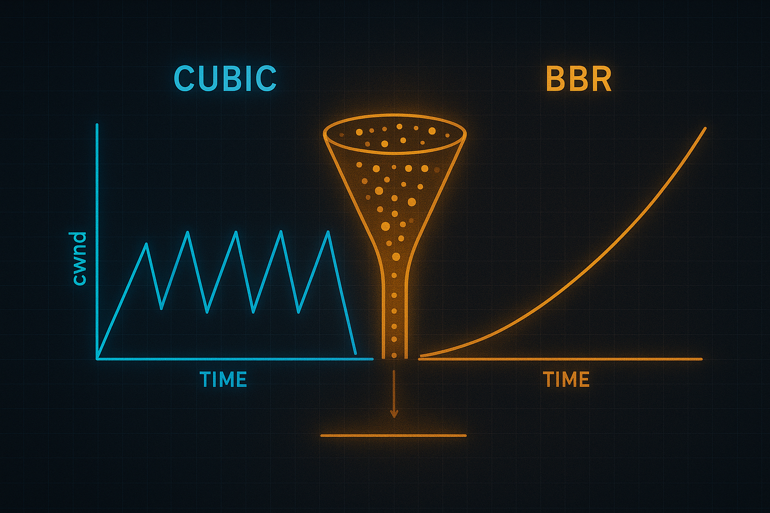
6.4 BBR vs. CUBIC
Scenario: 100 Mbps link, 50 ms RTT, 1 MB buffer

CUBIC behavior:
- Fills the buffer before loss
- Latency: 50 ms + 80 ms (buffer) = 130 ms
- Throughput: ~95 Mbps (after recovery overhead)
- Pattern: Sawtooth with periodic drops

BBR behavior:
- Targets 1 BDP in flight
- Latency: 50 ms + ~5 ms (minimal queue) ≈ 55 ms
- Throughput: ~98 Mbps
- Pattern: Steady with small variations
6.5 BBRv2 Improvements
BBRv2 (2019+) addresses fairness issues:
class BBRv2:
    def __init__(self):
        super().__init__()
        self.inflight_lo = inf  # Low watermark
        self.inflight_hi = inf  # High watermark
        self.loss_in_round = False

    def on_loss(self):
        """React to loss more like CUBIC."""
        self.inflight_hi = self.inflight * 0.85
        self.btl_bw = self.btl_bw * 0.9  # Reduce estimate

    def bound_cwnd(self):
        """Bound cwnd based on loss signals."""
        self.cwnd = min(self.cwnd, self.inflight_hi)
BBRv2 improves coexistence with loss-based flows like CUBIC.
7. Data Center Congestion Control
Data centers have unique requirements: low latency, high throughput, incast handling.
7.1 DCTCP (Data Center TCP)
DCTCP uses ECN (Explicit Congestion Notification) for fine-grained control:
class DCTCP:
    def __init__(self):
        self.cwnd = MSS
        self.alpha = 1  # Congestion estimate
        self.g = 0.0625  # Smoothing factor

    def on_ack(self, ecn_marked):
        if ecn_marked:
            self.marked_bytes += self.acked_bytes
        self.total_bytes += self.acked_bytes

        # At the end of a window
        if self.window_complete():
            # Fraction of marked packets
            F = self.marked_bytes / self.total_bytes

            # Update congestion estimate
            self.alpha = (1 - self.g) * self.alpha + self.g * F

            # Reduce cwnd proportionally
            self.cwnd = self.cwnd * (1 - self.alpha / 2)

            self.marked_bytes = 0
            self.total_bytes = 0
DCTCP achieves:
- Near-zero queue at switches
- High burst tolerance
- Sub-millisecond latency
7.2 HPCC (High Precision Congestion Control)
HPCC uses in-network telemetry for precise control:
class HPCC:
    def __init__(self):
        self.rate = initial_rate
        self.eta = 0.95  # Target utilization

    def on_ack(self, int_info):
        """
        int_info contains per-hop telemetry:
        - Link utilization
        - Queue length
        - Timestamp
        """
        max_utilization = 0

        for hop in int_info.hops:
            # Calculate utilization at this hop
            util = hop.tx_bytes / hop.bandwidth / hop.interval
            max_utilization = max(max_utilization, util)

        # Adjust rate based on most congested hop
        if max_utilization > self.eta:
            self.rate = self.rate * self.eta / max_utilization
        else:
            self.rate = self.rate + self.additive_increase
HPCC requires switch support but achieves optimal performance.
7.3 Swift
Swift (2020, Google) targets microsecond-scale latency:
class Swift:
    def __init__(self):
        self.cwnd = initial_cwnd
        self.target_delay = 10  # microseconds!

    def on_ack(self, fabric_delay):
        """
        fabric_delay = measured RTT - processing delay
        Pure network queuing delay
        """
        if fabric_delay < self.target_delay:
            # Below target: increase
            self.cwnd += self.ai_factor
        else:
            # Above target: decrease proportionally
            excess = (fabric_delay - self.target_delay) / fabric_delay
            self.cwnd = self.cwnd * (1 - excess * self.md_factor)
Swift achieves single-digit microsecond tail latencies.
8. Congestion Control for Special Networks
Different network environments require different approaches.
8.1 Satellite Networks
High latency, high bandwidth, long feedback loop:
GEO Satellite:
- RTT: 600 ms
- Bandwidth: 100 Mbps
- BDP: 7.5 MB

Challenge: Slow start takes forever!
Standard slow start: log₂(BDP/MSS) RTTs = ~13 RTTs = 8 seconds!
Solutions:
class SatelliteTCP:
    def __init__(self):
        # Higher initial cwnd
        self.cwnd = 10 * MSS  # RFC 6928

        # More aggressive slow start
        self.slow_start_multiplier = 2.89  # Like BBR

    def slow_start(self):
        # Faster ramp-up for high-BDP paths
        self.cwnd = self.cwnd * self.slow_start_multiplier
8.2 Wireless Networks
Wireless has non-congestion loss:
Challenges:
- Bit errors cause packet loss
- Handoffs cause temporary disconnection
- Variable link rates

Loss-based algorithms: interpret all loss as congestion → underutilization
Approaches:
def is_congestion_loss(self, loss_info):
    """Distinguish congestion from wireless loss."""
    # ECN marked = definitely congestion
    if loss_info.ecn_marked:
        return True

    # RTT spike = likely congestion
    if self.rtt > 2 * self.base_rtt:
        return True

    # Random single loss = likely wireless
    if loss_info.consecutive_losses == 1:
        return False

    return True  # Default to congestion
8.3 Cellular Networks
Cellular networks have deep buffers and variable capacity:
class CellularAware:
    def __init__(self):
        self.cwnd = MSS
        self.buffer_target = 100_ms  # Target buffer delay

    def on_ack(self, rtt, throughput):
        # Estimate buffer occupancy
        buffer_delay = rtt - self.min_rtt

        if buffer_delay > self.buffer_target:
            # Too much buffering
            self.cwnd = self.cwnd * 0.9
        elif throughput > self.estimated_capacity * 0.95:
            # Near capacity, gentle increase
            self.cwnd += MSS / self.cwnd
        else:
            # Below capacity, faster increase
            self.cwnd += MSS
9. Fairness and Coexistence
Congestion control algorithms must play well with others.
9.1 Fairness Metrics
def jain_fairness_index(rates):
    """
    Jain's fairness index: 1 = perfect fairness, 1/n = worst.
    """
    n = len(rates)
    sum_rates = sum(rates)
    sum_squares = sum(r ** 2 for r in rates)

    return (sum_rates ** 2) / (n * sum_squares)

# Example
flows = [50, 50, 50, 50]  # Mbps each
jfi = jain_fairness_index(flows)  # = 1.0 (perfect)

flows = [190, 5, 3, 2]  # One flow dominates
jfi = jain_fairness_index(flows)  # = 0.25 (unfair)
9.2 RTT Fairness
Flows with different RTTs get different throughput:
CUBIC with equal loss rate:
- Flow A: RTT = 10 ms → throughput = 100 Mbps
- Flow B: RTT = 100 ms → throughput = 31 Mbps

RTT unfairness ratio: 100/31 ≈ 3.2:1

CUBIC is actually RTT-fair to first approximation
because cwnd increases per RTT are similar.
BBR is more RTT-fair because it targets BDP directly.
9.3 Inter-Protocol Fairness
Different algorithms compete unequally:
CUBIC vs. Reno:
- CUBIC is more aggressive
- CUBIC tends to get more bandwidth

BBR vs. CUBIC:
- BBR keeps lower queues
- CUBIC fills buffers, sometimes starving BBR
- BBRv2 addresses this

Delay-based vs. Loss-based:
- Loss-based fills buffers
- Delay-based backs off when buffer fills
- Delay-based gets starved
9.4 The Deployment Challenge
New algorithms must coexist with existing traffic:
def safe_to_deploy(new_algorithm):
    """Criteria for deploying new congestion control."""
    tests = [
        # Doesn't harm existing traffic
        test_fairness_with_cubic(new_algorithm),
        test_fairness_with_reno(new_algorithm),

        # Doesn't cause congestion collapse
        test_stability_under_load(new_algorithm),

        # Converges to fair share
        test_convergence_time(new_algorithm),

        # Handles realistic conditions
        test_with_variable_capacity(new_algorithm),
        test_with_random_loss(new_algorithm),
    ]

    return all(tests)
10. Implementing Congestion Control
10.1 Linux TCP Stack
Linux allows pluggable congestion control:
# List available algorithms
sysctl net.ipv4.tcp_available_congestion_control
# cubic reno bbr

# Set default algorithm
sysctl -w net.ipv4.tcp_congestion_control=bbr

# Enable BBR (requires fq qdisc for pacing)
tc qdisc replace dev eth0 root fq
Kernel implementation interface:
struct tcp_congestion_ops {
    struct list_head list;
    char name[TCP_CA_NAME_MAX];

    // Required callbacks
    void (*init)(struct sock *sk);
    void (*cong_avoid)(struct sock *sk, u32 ack, u32 acked);
    u32  (*ssthresh)(struct sock *sk);

    // Optional callbacks
    void (*cwnd_event)(struct sock *sk, enum tcp_ca_event ev);
    void (*pkts_acked)(struct sock *sk, const struct ack_sample *sample);
    u32  (*undo_cwnd)(struct sock *sk);

    // Pacing support
    void (*set_rate)(struct sock *sk, u64 bw, int gain);
};
10.2 Userspace Congestion Control
QUIC enables userspace implementation:
class QUICCongestionControl:
    """QUIC allows per-connection congestion control."""

    def __init__(self, algorithm='cubic'):
        if algorithm == 'cubic':
            self.controller = CUBIC()
        elif algorithm == 'bbr':
            self.controller = BBR()

    def on_packet_sent(self, packet):
        self.bytes_in_flight += packet.size

    def on_ack_received(self, ack_frame):
        for packet in ack_frame.acked_packets:
            self.bytes_in_flight -= packet.size
            rtt = now() - packet.sent_time

            self.controller.on_ack(
                delivered=packet.size,
                rtt=rtt,
                inflight=self.bytes_in_flight
            )

    def on_packet_lost(self, packet):
        self.bytes_in_flight -= packet.size
        self.controller.on_loss()

    def can_send(self):
        return self.bytes_in_flight < self.controller.cwnd
10.3 Debugging Congestion Control
# Monitor TCP state
ss -tin | grep -A2 "10.0.0.1"
# Shows: cwnd, rtt, retransmits, pacing_rate

# Trace congestion control events
perf trace -e 'tcp:*' -- curl https://example.com

# Visualize with tcptrace
tcptrace -G input.pcap
# Generates time-sequence graphs
# Programmatic monitoring
import socket

def get_tcp_info(sock):
    """Get TCP congestion control state."""
    TCP_INFO = 11
    info = sock.getsockopt(socket.IPPROTO_TCP, TCP_INFO, 200)

    # Parse tcp_info struct
    state, ca_state, retransmits, probes, backoff, options, \
    snd_wscale_rcv_wscale, delivery_rate_app_limited, \
    rto, ato, snd_mss, rcv_mss, \
    unacked, sacked, lost, retrans, fackets, \
    last_data_sent, last_ack_sent, last_data_recv, last_ack_recv, \
    pmtu, rcv_ssthresh, rtt, rttvar, snd_ssthresh, snd_cwnd, \
    advmss, reordering = struct.unpack('BBBBBBBBIIIIIIIIIIIIIIIIIII', info[:104])

    return {
        'cwnd': snd_cwnd,
        'ssthresh': snd_ssthresh,
        'rtt': rtt,  # microseconds
        'retransmits': retrans,
    }
11. Real-World Debugging and Optimization
11.1 Diagnosing Congestion Issues
When applications perform poorly, congestion control is often the culprit:
# Check current algorithm and state
ss -tin dst 10.0.0.1:443
# Output:
# cubic wscale:7,7 rto:204 rtt:15.2/3.1 mss:1448 pmtu:1500
# rcvmss:1448 advmss:1448 cwnd:42 ssthresh:35 bytes_sent:1234567
# bytes_acked:1234000 segs_out:1000 segs_in:950 data_segs_out:990
# send 39.5Mbps lastsnd:4 lastrcv:4 lastack:4 pacing_rate 47.3Mbps
# delivery_rate 38.2Mbps busy:2000ms retrans:0/5 dsack_dups:2
# rcv_rtt:15 rcv_space:29200 rcv_ssthresh:65535

# Key metrics to watch:
# - cwnd vs ssthresh: are we in slow start or congestion avoidance?
# - retrans: how many retransmissions?
# - rtt vs rto: is RTO appropriate for the RTT?
# - send vs delivery_rate: are we limited by congestion control?
11.2 Common Performance Problems
Problem: Slow start taking too long
Symptoms: First few seconds of transfer are slow
Cause: cwnd starts small, takes many RTTs to grow
Solution:
- Increase initial cwnd (Linux default is 10 segments)
- Use TCP Fast Open to save RTT
- Persistent connections to reuse established cwnd

Problem: Stuck in slow start
Symptoms: Never reaches full throughput
Cause: ssthresh set too low from previous loss
Solution: Check for packet loss, buffer issues, or algorithm bugs

Problem: Sawtooth too aggressive
Symptoms: High throughput with periodic drops and latency spikes
Cause: CUBIC filling buffers before loss detection
Solution: Switch to BBR, enable ECN, or tune CUBIC parameters

Problem: Poor performance on high-latency links
Symptoms: Low throughput despite no loss
Cause: cwnd not growing fast enough for large BDP
Solution: Use algorithm tuned for high BDP (BBR, HTCP, or tuned CUBIC)
11.3 Algorithm Selection Guide
def recommend_algorithm(network_conditions):
    """Recommend congestion control algorithm based on conditions."""

    if network_conditions.type == 'data_center':
        if network_conditions.has_ecn:
            return 'DCTCP'
        elif network_conditions.has_int:
            return 'HPCC'
        else:
            return 'BBR'

    if network_conditions.type == 'wan':
        if network_conditions.rtt > 100:  # ms
            return 'BBR'  # Better for high-latency
        elif network_conditions.has_deep_buffers:
            return 'BBR'  # Avoids bufferbloat
        else:
            return 'CUBIC'  # Good general-purpose

    if network_conditions.type == 'wireless':
        return 'BBR'  # Better handles non-congestion loss

    if network_conditions.type == 'satellite':
        return 'Hybla' or 'BBR'  # Designed for high-latency

    return 'CUBIC'  # Safe default
11.4 Tuning for Specific Workloads
# For bulk transfers (maximize throughput)
sysctl -w net.ipv4.tcp_congestion_control=bbr
sysctl -w net.core.rmem_max=134217728
sysctl -w net.core.wmem_max=134217728
sysctl -w net.ipv4.tcp_rmem="4096 87380 134217728"
sysctl -w net.ipv4.tcp_wmem="4096 65536 134217728"

# For latency-sensitive (minimize delay)
sysctl -w net.ipv4.tcp_congestion_control=bbr
sysctl -w net.ipv4.tcp_notsent_lowat=16384
tc qdisc replace dev eth0 root fq

# For many short connections
sysctl -w net.ipv4.tcp_slow_start_after_idle=0
sysctl -w net.ipv4.tcp_fastopen=3
sysctl -w net.ipv4.tcp_tw_reuse=1
11.5 Monitoring and Alerting
class CongestionMonitor:
    """Monitor congestion control health across connections."""

    def __init__(self):
        self.thresholds = {
            'retransmit_rate': 0.01,  # 1% is concerning
            'rtt_increase': 2.0,      # 2x baseline is concerning
            'throughput_drop': 0.5,   # 50% of expected is concerning
        }

    def check_connection(self, conn_stats):
        alerts = []

        # Check retransmission rate
        retrans_rate = conn_stats.retrans / conn_stats.segs_out
        if retrans_rate > self.thresholds['retransmit_rate']:
            alerts.append(f"High retransmit rate: {retrans_rate:.2%}")

        # Check RTT inflation (bufferbloat)
        if conn_stats.rtt > conn_stats.min_rtt * self.thresholds['rtt_increase']:
            alerts.append(f"RTT inflated: {conn_stats.rtt}ms vs {conn_stats.min_rtt}ms baseline")

        # Check throughput
        expected = conn_stats.cwnd * 8 / (conn_stats.rtt / 1000)  # bits/sec
        if conn_stats.delivery_rate < expected * self.thresholds['throughput_drop']:
            alerts.append(f"Throughput below expected: {conn_stats.delivery_rate} vs {expected}")

        return alerts

    def aggregate_metrics(self, all_connections):
        """Aggregate metrics across all connections for dashboards."""
        return {
            'median_rtt': statistics.median(c.rtt for c in all_connections),
            'p99_rtt': statistics.quantiles([c.rtt for c in all_connections], n=100)[98],
            'total_retransmits': sum(c.retrans for c in all_connections),
            'connections_in_slow_start': sum(1 for c in all_connections if c.cwnd < c.ssthresh),
            'avg_cwnd': statistics.mean(c.cwnd for c in all_connections),
        }
12. Historical Context and Future Directions
12.1 The Evolution of Congestion Control
Timeline of Major Developments:

1986: Congestion collapse observed
1988: Jacobson's algorithms (Tahoe) - saved the Internet
1990: Reno with fast recovery
1994: Vegas (delay-based, ahead of its time)
1999: NewReno (multiple loss recovery)
2004: BIC (predecessor to CUBIC)
2006: CUBIC (Linux default)
2008: Compound TCP (Windows default)
2010: DCTCP (data center revolution)
2016: BBR v1 (model-based paradigm shift)
2019: BBR v2 (fairness improvements)
2020+: Swift, HPCC (microsecond-scale latency)
12.2 Emerging Trends
Machine Learning for Congestion Control:
class LearnedCongestionControl:
    """Use reinforcement learning to optimize congestion control."""

    def __init__(self):
        self.model = load_trained_model('congestion_rl.pt')
        self.state_buffer = []

    def get_state(self, conn):
        """Extract features for ML model."""
        return [
            conn.cwnd / conn.mss,
            conn.rtt / 1000,
            conn.rtt / conn.min_rtt,
            conn.delivery_rate,
            conn.loss_rate,
            conn.inflight / conn.cwnd,
        ]

    def decide_action(self, state):
        """ML model outputs cwnd adjustment."""
        with torch.no_grad():
            action = self.model(torch.tensor(state))

        # Action space: [-0.5, -0.1, 0, 0.1, 0.5] multipliers
        return action.argmax().item()

    def on_ack(self, conn):
        state = self.get_state(conn)
        action = self.decide_action(state)

        # Apply action
        multipliers = [0.5, 0.9, 1.0, 1.1, 1.5]
        conn.cwnd = int(conn.cwnd * multipliers[action])
Research systems like Orca, PCC, and Aurora use ML for congestion control.
Programmable Data Planes:
P4-based congestion control:
- Switches can compute and signal congestion precisely
- Enable algorithms impossible with end-to-end signals
- Examples: HPCC, NDP, pHost

Benefits:
- Faster reaction (switch vs. RTT timescale)
- More accurate information (exact queue lengths)
- New algorithm designs possible
Multi-Path Congestion Control:
class MPTCPCongestionControl:
    """Congestion control for multi-path TCP."""

    def __init__(self, subflows):
        self.subflows = subflows

    def coupled_increase(self):
        """
        Linked Increases Algorithm (LIA):
        Increase on best path, but total increase <= single-path.
        """
        max_cwnd_rtt = max(sf.cwnd / sf.rtt for sf in self.subflows)

        for sf in self.subflows:
            # Increase proportional to path quality
            alpha = self.compute_alpha()
            sf.cwnd += alpha * sf.mss * sf.mss / sf.cwnd

    def compute_alpha(self):
        """Compute coupled increase parameter."""
        sum_cwnd_rtt = sum(sf.cwnd / sf.rtt for sf in self.subflows)
        max_cwnd_rtt = max(sf.cwnd / sf.rtt for sf in self.subflows)
        sum_cwnd = sum(sf.cwnd for sf in self.subflows)

        return sum_cwnd * max_cwnd_rtt / (sum_cwnd_rtt ** 2)
12.3 Open Challenges
Challenge 1: Fairness at Scale
- Billions of flows competing
- No global coordination
- Different algorithms coexisting

Challenge 2: Edge Networks
- Highly variable capacity
- Mixed wired/wireless paths
- Deep buffers cause bloat

Challenge 3: Low Latency Requirements
- AR/VR needs < 10ms latency
- Gaming needs consistent timing
- Traditional CC too slow to react

Challenge 4: Privacy
- Congestion signals leak information
- Encrypted traffic still reveals patterns
- Need privacy-preserving algorithms

Challenge 5: Verification
- Can't test all network conditions
- Formal verification hard for dynamic systems
- Deployment risks with new algorithms
13. Summary
TCP congestion control has evolved dramatically over four decades:
Classic algorithms:
- Tahoe/Reno: Loss as the signal, AIMD dynamics
- NewReno: Better handling of multiple losses
- CUBIC: Aggressive probing with cubic function
Delay-based algorithms:
- Vegas: RTT increase as early warning
- FAST: High-speed network optimization
- Compound: Hybrid loss + delay approach
Model-based algorithms:
- BBR: Explicit bandwidth and RTT estimation
- BBRv2: Better fairness with loss-based flows
Data center algorithms:
- DCTCP: ECN-based fine-grained control
- HPCC: In-network telemetry
- Swift: Microsecond-scale latency
Key takeaways:
- No single algorithm is best: Different networks need different approaches
- Fairness is hard: Algorithms must coexist with existing traffic
- Latency matters: Bufferbloat is a real problem that BBR addresses
- The network is evolving: New capabilities (ECN, INT) enable new algorithms
- Deployment is challenging: Must work with the installed base
- Measurement is essential: You can’t optimize what you don’t measure
- History repeats: Ideas from Vegas (1995) reappear in modern algorithms
Understanding congestion control is essential for anyone building networked systems. Whether you’re diagnosing performance problems, choosing algorithms for your infrastructure, or building new protocols, this knowledge is foundational to effective network engineering. The algorithms running on your computer right now are the result of decades of research, countless experiments, and hard-won lessons from production deployments.