The PCP Theorem: Why Some Problems Are Hard Even to Approximate
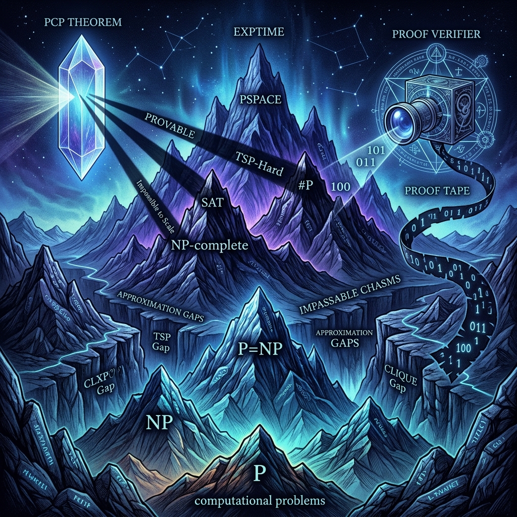
Unpack one of theoretical computer science's crown jewels: the PCP theorem, which shows that for many NP-hard problems, even finding an approximate solution is intractable — and how probabilistically checkable proofs revolutionized our understanding of hardness.
Contents
Consider the following scenario: a brilliant but untrustworthy oracle claims to have a proof that a given 3-SAT formula is satisfiable. You are skeptical. You want to verify the proof, but the proof is enormous — far too long for you to read in its entirety. What if you could randomly sample just a constant number of bits from the proof, and based on those few bits, decide with high confidence whether the proof is valid? The PCP theorem — one of the deepest and most surprising results in theoretical computer science — says that this is possible. More precisely, (\mathbf{NP} = \mathbf{PCP}[O(\log n), O(1)]): every language in NP has a probabilistically checkable proof that can be verified by reading only a constant number of bits, using (O(\log n)) random bits to choose which bits to read.
This result, proved by Arora, Safra, Arora, Lund, Motwani, Sudan, and Szegedy in the early 1990s, fundamentally changed our understanding of computational complexity. Its most dramatic consequence is the hardness of approximation: for many NP-hard optimization problems, not only is finding the exact optimum intractable, but even finding an approximate solution within certain factors is intractable. Before the PCP theorem, we had no systematic way of proving that approximation is hard. After the PCP theorem, an entire landscape of inapproximability results emerged, transforming the field of approximation algorithms.
This article will take you through the intellectual journey of the PCP theorem: the motivation from approximation algorithms, the statement and its intuitive meaning, the high-level structure of the proof (algebraic approach, low-degree testing, composition), the consequences for specific optimization problems, and the modern frontier — the Unique Games Conjecture and its implications. We will not shy away from the technical details, but our focus will be on building deep intuition for why this theorem is true and why it matters.
1. Motivation: approximation algorithms and the gap
Before the PCP theorem, theoretical computer scientists studied approximation algorithms on a problem-by-problem basis. For some NP-hard problems, efficient approximation algorithms existed with excellent guarantees. For others, no such algorithms were known, and researchers could only prove NP-hardness of exact solution — leaving open the possibility that a good approximation might exist.
1.1 The landscape of approximation
Consider three canonical optimization problems:
Knapsack: Given items with weights and values, and a capacity, find the subset of maximum total value that fits within the capacity. Knapsack admits a fully polynomial-time approximation scheme (FPTAS): for any (\varepsilon > 0), there is an algorithm that runs in time polynomial in (n) and (1/\varepsilon) and achieves a ((1 + \varepsilon))-approximation (or ((1 - \varepsilon)) for the maximization version).
Minimum Vertex Cover: Given a graph, find the smallest set of vertices that touches every edge. Vertex Cover admits a simple 2-approximation (take all endpoints of a maximal matching) and is APX-complete. Kannan and later Dinur and Safra showed it is NP-hard to approximate within any factor better than (\sqrt{2}) (and assuming the Unique Games Conjecture, within any factor better than 2).
Maximum Clique: Given a graph, find the largest complete subgraph. This problem is dramatically harder to approximate. Håstad’s celebrated result (1996) showed that, assuming (\mathbf{P} \neq \mathbf{NP}), Maximum Clique cannot be approximated within a factor of (n^{1-\varepsilon}) for any (\varepsilon > 0).
The question is: what accounts for this vast difference in approximability? Why does Knapsack have a PTAS while Clique cannot even be approximated to within a polynomial factor?
1.2 PTAS, APX, and the gap problem
Let us formalize the classes of approximation. Let (\mathcal{P}) be an NP-hard optimization problem. We say:
- (\mathcal{P} \in \mathbf{PTAS}) if for every (\varepsilon > 0), there is a polynomial-time ((1 + \varepsilon))-approximation algorithm (or ((1 - \varepsilon)) for maximization).
- (\mathcal{P} \in \mathbf{APX}) if there is a constant-factor approximation algorithm.
- (\mathcal{P}) is (\mathbf{APX})-hard if every problem in APX reduces to it via an approximation-preserving reduction.
- (\mathcal{P} \in \mathbf{FPTAS}) if there is a PTAS whose running time is polynomial in both (n) and (1/\varepsilon).
The gap between PTAS and APX-hardness is where the PCP theorem does its work. To prove that a problem has no PTAS (unless (\mathbf{P} = \mathbf{NP})), it suffices to exhibit a “gap-producing reduction”: a polynomial-time reduction from an NP-complete problem that creates a gap between YES-instances and NO-instances. Specifically, the reduction maps:
- YES-instances of the NP-complete problem to instances of (\mathcal{P}) with optimal value at least (c).
- NO-instances of the NP-complete problem to instances of (\mathcal{P}) with optimal value at most (s).
If (c/s) is some constant (\rho > 1), then approximating the problem within a factor better than (\rho) would distinguish YES from NO instances, solving the NP-complete problem. This is called a “gap-introducing reduction,” and the PCP theorem provides a systematic way of constructing such reductions.
2. The PCP theorem statement and its meaning
The PCP theorem can be stated concisely:
[ \mathbf{NP} = \mathbf{PCP}[O(\log n), O(1)] ]
But what does this notation mean?
2.1 The PCP model
A probabilistically checkable proof (PCP) system for a language (L) consists of a probabilistic polynomial-time verifier (V) that, given an input (x) and oracle access to a proof string (\pi), works as follows:
- (V) reads (x) and flips (r(n)) random coins to generate a random string (R).
- Based on (x) and (R), (V) generates a list of (q(n)) positions in the proof (\pi).
- (V) queries those positions (reads those bits of (\pi)) and decides to accept or reject.
The class (\mathbf{PCP}[r(n), q(n)]) is the set of languages for which there exists a verifier using (O(r(n))) random bits and (O(q(n))) queries satisfying:
- Completeness: If (x \in L), then there exists a proof (\pi) such that (\Pr[V^{\pi}(x) \text{ accepts}] = 1).
- Soundness: If (x \notin L), then for every proof (\pi), (\Pr[V^{\pi}(x) \text{ accepts}] \leq 1/2).
The PCP theorem asserts that every language in NP has a PCP verifier that uses (O(\log n)) random bits and reads only (O(1)) bits of the proof. The number of possible random strings is (2^{O(\log n)} = \text{poly}(n)), so the verifier’s decision can be computed in polynomial time.
2.2 Intuition: encoding the NP witness
How can this possibly work? Suppose (L \in \mathbf{NP}). Then there is a polynomial-time verifier (V_{\text{NP}}) that, given an input (x) and a witness (w), checks whether (w) is a valid proof that (x \in L). The naive way to turn this into a PCP would be to give the verifier the entire witness (w) and have it check one random clause of the verification circuit. But reading a random clause might require looking at many bits.
The magic of the PCP theorem is that there is a way to encode the witness (w) into a much longer, highly redundant proof (\pi) such that:
- If (w) is a valid witness, (\pi) is a valid encoding that will be accepted with probability 1.
- If no valid witness exists, then every string (\pi) will be rejected with probability at least (1/2), and the rejection can be detected by looking at only a constant number of bits.
The encoding is based on algebraic techniques: the witness is represented as a multivariate polynomial over a finite field, and the PCP verifier checks that this polynomial satisfies certain properties at randomly chosen points. The redundancy of the polynomial encoding ensures that any “invalid proof” must deviate from the correct polynomial in a way that is detectable by a constant number of random queries.
2.3 The trivial direction: PCP[O(log n), O(1)] ⊆ NP
One direction of the equality is relatively straightforward. Given a PCP verifier using (O(\log n)) random coins, we can enumerate all (2^{O(\log n)} = \text{poly}(n)) possible random strings. For each random string, we can enumerate all possible query answers (there are only (2^{O(1)} = O(1)) possible answer patterns). The NP witness is simply a satisfying assignment of query answers for all random strings: the witness provides, for each random string, the answers to the queries, and the NP verifier checks that these answers are consistent and lead to acceptance. This shows (\mathbf{PCP}[O(\log n), O(1)] \subseteq \mathbf{NP}). The difficult direction is (\mathbf{NP} \subseteq \mathbf{PCP}[O(\log n), O(1)]).
3. The algebraic approach: a proof sketch
The proof of the PCP theorem is one of the most complex in all of computer science. We cannot present a full proof here (Arora and Barak’s textbook devotes over 60 pages to it), but we can sketch the main ideas at a high level, focusing on the intuition.
3.1 Step 1: Arithmetization
The starting point is an NP-complete problem expressed in a convenient form. A canonical choice is the constraint satisfaction problem (CSP) — specifically, 3-SAT or, more generally, the problem of checking whether a given Boolean circuit is satisfiable. The first step is to “arithmetize” the computation: represent the NP verification procedure as a system of algebraic equations over a finite field.
Given a Boolean formula (\varphi) with (n) variables and (m) clauses, we can represent the satisfying assignments as the solutions to a set of polynomial equations. For each clause ((x_i \lor \neg x_j \lor x_k)), we write a polynomial equation like:
[ (1 - x_i) \cdot x_j \cdot (1 - x_k) = 0 ]
over the field (\mathbb{F}_2) (or a larger field for technical reasons). The arithmetization extends the Boolean formula to a low-degree multivariate polynomial (P) over a finite field (\mathbb{F}) such that (\varphi) is satisfiable if and only if there exists an assignment (a \in {0, 1}^n) with (P(a) = 0) (or, in some constructions, with (P) evaluating to 0 at all points in a certain set).
3.2 Step 2: Low-degree extension
The next key idea is the low-degree extension (LDE). Instead of having the prover supply the assignment directly, we ask the prover to supply a multivariate polynomial (f : \mathbb{F}^m \to \mathbb{F}) of low degree that extends the assignment. Specifically, the assignment to the (n) variables is encoded as the values of (f) on a subset (H^m \subset \mathbb{F}^m) (where (H = {0, 1}) or a small subset). The polynomial has degree at most (|H| - 1) in each variable, so its total degree is bounded.
The crucial property is that any two distinct low-degree polynomials agree on at most a small fraction of points (this follows from the Schwartz-Zippel lemma). Therefore, if a prover supplies a polynomial that is “mostly correct” — that agrees with the true low-degree extension on most points — then it must be the exact correct polynomial, or the verifier will catch the discrepancy with high probability by querying a random point.
3.3 Step 3: The sum-check protocol
The verifier needs to check that the low-degree polynomial (f) encodes a satisfying assignment. This involves checking that certain equations hold for all points in (H^m). The sum-check protocol (introduced by Lund, Fortnow, Karloff, and Nisan in 1990) allows a verifier to check sums of the form:
[ \sum*{x_1 \in H} \sum*{x2 \in H} \dots \sum{x_m \in H} g(x_1, \dots, x_m) ]
by asking the prover for evaluations of certain low-degree polynomials at randomly chosen points. The protocol reduces the task of verifying a sum over exponentially many points to verifying a single evaluation of a polynomial at a random point. Crucially, the verifier only needs to query the prover for (O(m)) values — and (m) can be made polylogarithmic using techniques like degree reduction.
3.4 Step 4: Low-degree testing
How does the verifier know that the string (\pi) it is querying actually represents a low-degree polynomial? The verifier performs a low-degree test: it queries a few points of (\pi) and checks that they are consistent with some low-degree polynomial. The fundamental result (the “low-degree test,” proved by Rubinfeld and Sudan, building on work by Babai, Fortnow, and Lund) states that if a function (f) passes a low-degree test with sufficiently high probability, then (f) is close to some low-degree polynomial (g) (in Hamming distance). The verifier can then reason about (g) even though it only queries (f).
3.5 Step 5: Composition (or “proof recursion”)
The original proof of the PCP theorem by Arora and Safra, and the streamlined version by Arora, Lund, Motwani, Sudan, and Szegedy, used a technique called composition (also known as “proof recursion” or the “booster”). The idea is:
- Start with a PCP verifier that uses (O(\log n)) randomness and (O(\log n)) queries (relatively easy to construct from arithmetization).
- Apply a “composition lemma” that reduces the query complexity from (O(\log n)) to (O(1)), while preserving the randomness bound of (O(\log n)).
The composition lemma works by taking the verification procedure of the “outer” verifier and expressing it as a 3-SAT formula (or similar CSP) of polylogarithmic size. Then an “inner” PCP verifier is applied to this CSP, reducing the number of queries to a constant. The composition of the two verifiers yields the desired (\mathbf{PCP}[O(\log n), O(1)]) verifier.
Irit Dinur (2006) later gave a dramatically different proof of the PCP theorem using gap amplification via expander graphs. Her proof is more combinatorial and arguably more intuitive: start with a trivial PCP (where the verifier reads the entire proof) and iteratively amplify the gap between completeness and soundness while maintaining the query complexity. Each iteration uses expander walks to “spread out” the queries. Dinur’s proof is considered one of the most beautiful achievements in modern complexity theory.
4. Consequences: the inapproximability landscape
With the PCP theorem in hand, we can prove strong inapproximability results for a wide variety of optimization problems. The general recipe is:
- Start with a PCP verifier for an NP-complete language.
- Construct a “PCP-to-gap” reduction: for each random string, create a constraint (or “test”) that checks the verifier’s acceptance condition.
- Map YES instances to optimization instances with high optimum, and NO instances to instances with low optimum, creating a gap.
4.1 Max-3SAT
Max-3SAT is the optimization version of 3-SAT: given a 3-CNF formula, find an assignment that maximizes the number of satisfied clauses. The PCP theorem directly implies that there exists a constant (\varepsilon > 0) such that approximating Max-3SAT within a factor of (1 + \varepsilon) is NP-hard. Later work by Håstad (2001) pinned down the exact threshold: for any (\varepsilon > 0), it is NP-hard to distinguish 3-SAT instances where a ((7/8 + \varepsilon)) fraction of clauses can be satisfied from those where at most a (7/8) fraction can be. The factor (7/8) is tight, since a random assignment satisfies (7/8) of the clauses in expectation, and this can be derandomized (Karloff-Zwick gives a (7/8)-approximation).
4.2 Maximum Clique
The connection between PCPs and clique approximation goes through the FGLSS reduction (Feige, Goldwasser, Lovász, Safra, and Szegedy, 1991). Given a PCP verifier, we construct a graph as follows:
- Vertices correspond to pairs (random string (R), query answers consistent with acceptance).
- Two vertices are connected if they are “consistent” — i.e., they agree on the values of any queries they share.
A valid proof (\pi) corresponds to a large clique in this graph: the set of all (random string, answers-from-(\pi)) pairs. Conversely, a large clique can be decoded into a proof that makes the verifier accept with high probability. The FGLSS reduction transforms a PCP with completeness (1) and soundness (s) into a gap instance of Maximum Clique: YES instances produce graphs with a clique of size at least (C), and NO instances produce graphs where the maximum clique is at most (S), with (C/S \approx 1/s).
By varying the parameters of the PCP, different inapproximability ratios can be achieved. Håstad’s (n^{1-\varepsilon}) hardness for Clique uses a PCP with extremely low soundness (roughly (n^{-1+\varepsilon})), achieved by iterated parallel repetition combined with algebraic techniques.
4.3 Set Cover
Set Cover is another classical NP-hard problem: given a universe (U) and a family of sets (\mathcal{S} \subseteq 2^U), find the smallest subfamily that covers (U). Feige (1998) used the PCP theorem to show that Set Cover cannot be approximated within a factor of ((1 - \varepsilon) \ln n) for any (\varepsilon > 0), unless (\mathbf{NP} \subseteq \mathbf{DTIME}(n^{\log \log n})). This matches the approximation ratio achieved by the greedy algorithm (which is (\ln n)), showing that the greedy algorithm is essentially optimal.
The reduction maps a PCP verifier to a Set Cover instance where:
- The universe consists of the random strings on which the verifier accepts (with the right proof).
- Each possible proof bit position (and its value) defines a set covering all random strings whose queries are consistent with that proof bit.
The gap in the Set Cover instance corresponds to the gap between the proof length and the minimum number of proof bits needed to define a valid proof.
4.4 Label Cover and the Raz parallel repetition theorem
A central intermediate problem in PCP-based hardness reductions is Label Cover, introduced by Arora et al. Given a bipartite graph with constraints on edge labels (each vertex must be assigned a label from its alphabet, and constraints specify which label pairs are allowed on each edge), the goal is to find an assignment that maximizes the number of satisfied edges. Label Cover is the “canonical” PCP-hard problem: nearly all tight inapproximability results are obtained by reducing from Label Cover.
The Raz parallel repetition theorem (1998) is the key tool for amplifying the soundness of Label Cover (and thus of PCPs). Given a two-prover one-round proof system with soundness (s < 1), the (k)-fold parallel repetition has soundness (s^k). Raz proved that this exponential decrease is essentially tight, giving a precise characterization of how soundness behaves under parallel repetition. This theorem is the foundation for many strong inapproximability results.
5. Modern frontiers: the Unique Games Conjecture
The PCP theorem established that many problems are hard to approximate within some constant factor. But for many problems, the exact threshold of approximability remained open. The Unique Games Conjecture (UGC), proposed by Subhash Khot in 2002, aims to pin down these thresholds precisely.
5.1 Statement of the UGC
The Unique Games problem is a special case of Label Cover where the constraints on each edge are permutations (bijections between the label sets of the two vertices). In other words, for each edge ((u, v)) and each label of (u), there is exactly one label of (v) that satisfies the constraint. The Unique Games Conjecture asserts that, for any (\varepsilon, \delta > 0), there exists an alphabet size (k) such that it is NP-hard to distinguish between:
- YES: There is an assignment satisfying at least a (1 - \varepsilon) fraction of constraints.
- NO: Every assignment satisfies at most a (\delta) fraction of constraints.
Intuitively, Unique Games says: even when the constraints are extremely “easy” (in the sense that every partial assignment can be extended uniquely), it is still NP-hard to tell whether the instance is almost perfectly satisfiable or almost completely unsatisfiable.
5.2 Consequences of the UGC
Assuming the UGC, many important problems have been shown to have tight approximation thresholds:
- Vertex Cover: Hard to approximate within any factor better than 2 (matching the simple 2-approximation).
- Maximum Cut: Hard to approximate within any factor better than (\alpha_{\text{GW}} \approx 0.878) (matching the Goemans-Williamson SDP-based approximation).
- Sparsest Cut: Hard to approximate within any constant factor (resolving a long-standing open problem).
- Constraint Satisfaction Problems: For every CSP, the optimal approximation ratio equals the integrality gap of a natural SDP relaxation. This is Raghavendra’s result (2008): assuming the UGC, for every CSP, the best polynomial-time approximation is achieved by a specific semidefinite programming relaxation.
5.3 Status of the UGC
The Unique Games Conjecture remains unproven. Subexponential-time algorithms for Unique Games exist (Arora, Barak, and Steurer, 2015), showing that if the conjecture is true, the reduction must incur at least a quasipolynomial blowup. This does not refute the conjecture — which is about polynomial-time reductions — but it does constrain the form that a proof could take. The UGC is now considered one of the most important open problems in complexity theory, alongside (\mathbf{P}) vs (\mathbf{NP}).
6. Technical deep dive: the sum-check protocol
Let us now go deeper into one of the core technical components: the sum-check protocol. This protocol is a beautiful piece of interactive proof theory and illustrates the power of algebraic techniques in complexity theory.
6.1 The setting
We work over a finite field (\mathbb{F}). Let (g(x_1, \dots, x_m)) be an (m)-variate polynomial over (\mathbb{F}) of degree at most (d) in each variable. The verifier wants to check the claim that:
[ \sum*{x_1 \in {0,1}} \sum*{x2 \in {0,1}} \dots \sum{x_m \in {0,1}} g(x_1, \dots, x_m) = C ]
where (C \in \mathbb{F}) is some claimed value. Naively computing the sum requires evaluating (g) on all (2^m) Boolean inputs, which is exponentially large. The sum-check protocol allows the verifier to verify the claim using only (O(md)) field operations and queries to (g) at a single random point — provided the prover is cooperative.
6.2 The protocol
The protocol proceeds in (m) rounds. In round (i) ((i = 1, \dots, m)), the prover sends a univariate polynomial (h_i(z)) of degree at most (d), which is claimed to equal:
[ hi(z) = \sum{x*{i+1} \in {0,1}} \dots \sum*{xm \in {0,1}} g(r_1, \dots, r{i-1}, z, x_{i+1}, \dots, x_m) ]
where (r1, \dots, r{i-1}) are the random field elements chosen by the verifier in previous rounds.
The verifier then checks that:
[ hi(0) + h_i(1) = h{i-1}(r_{i-1}) ]
(with (h_0(r_0)) defined as (C)). If the check passes, the verifier picks a random (r_i \in \mathbb{F}) and sends it to the prover for the next round.
After (m) rounds, the verifier has a claim that (h_m(r_m) = g(r_1, \dots, r_m)). The verifier now queries the oracle for (g) at this single point and checks the equality.
6.3 Analysis
If the original sum claim is true, an honest prover can follow the protocol and the verifier will accept with probability 1 (completeness).
If the original sum claim is false, then no matter what the prover does, at least one round must involve a lie. In round (i), if the prover sends (hi) that is not the true partial sum polynomial, then with probability at least (1 - d/|\mathbb{F}|) over the choice of (r_i), the check (h_i(0) + h_i(1) = h{i-1}(r_{i-1})) or the subsequent consistency checks will fail. This is because two distinct degree-(d) univariate polynomials can agree on at most (d) points (by the fundamental theorem of algebra over finite fields). By making the field large enough (specifically, (|\mathbb{F}| \gg md)), the soundness error can be made arbitrarily small.
The sum-check protocol reduces the hard task of verifying an exponentially large sum to the easy task of checking a single evaluation, at the cost of (m) rounds of interaction. This “compression” of verification is the heart of interactive proofs and, by extension, of PCPs.
7. From PCP to inapproximability: a worked example
Let us walk through a concrete reduction to understand how the PCP theorem yields inapproximability. We will sketch the proof that Max-3SAT has no PTAS unless (\mathbf{P} = \mathbf{NP}).
7.1 The PCP verifier for 3-SAT
Start with the trivial NP verifier for 3-SAT: the witness is a satisfying assignment, and the verifier checks every clause. We apply the PCP theorem to transform this into a PCP verifier (V) that:
- Uses (O(\log n)) random coins, generating a random string (R).
- Queries (q = O(1)) bits of the proof (\pi).
- Based on the answers, decides to accept or reject.
The verifier’s decision for each random string (R) can be expressed as a Boolean function (f_R : {0, 1}^q \to {0, 1}): accept if the query answers satisfy (f_R).
7.2 Constructing a Max-3SAT instance
Now, for each possible random string (R), we construct a 3-CNF formula (\varphi_R) that encodes the constraint (f_R). This is always possible because any Boolean function on (q) bits can be expressed as a 3-CNF formula (possibly with auxiliary variables) of constant size, since (q) is constant. Specifically, we introduce variables (y_1, \dots, y_k) representing the proof bits (where (k) is the total number of distinct proof positions queried across all random strings). For each random string (R), (\varphi_R) takes the queried variables as inputs and is satisfied precisely when (f_R) accepts.
The Max-3SAT instance is the conjunction of all (\varphi_R) for all random strings. The number of clauses is (O(2^{O(\log n)} \cdot 2^q) = \text{poly}(n)).
7.3 The gap
Now consider the two cases:
If the original 3-SAT instance is satisfiable, then there exists a proof (\pi) (the PCP encoding of the satisfying assignment) such that (V) accepts on every random string. Setting the variables (y_i) according to (\pi), every clause in every (\varphi_R) is satisfied. So the Max-3SAT instance has an assignment satisfying all clauses.
If the original 3-SAT instance is unsatisfiable, then for every proof (\pi), the verifier rejects on at least half of the random strings. For any assignment to the variables (y_i), at least (1/2) of the (\varphi_R) formulas are unsatisfied. Since each (\varphi_R) has at least one clause, the fraction of unsatisfied clauses is at least (\varepsilon = 1/(2c)) for some constant (c) (accounting for the number of clauses per (\varphi_R)).
Thus, approximating Max-3SAT within a factor better than (1 - \varepsilon) would distinguish satisfiable from unsatisfiable 3-SAT instances, implying (\mathbf{P} = \mathbf{NP}).
7.4 The exact threshold: Håstad’s 3-bit PCP
The factor of (1 - \varepsilon) in the above argument is not tight. Håstad (2001) constructed a PCP where the verifier reads exactly 3 bits and accepts if they satisfy a linear equation modulo 2 (an XOR of 3 variables). The completeness is (1 - \varepsilon) (the verifier accepts with probability arbitrarily close to 1 on valid proofs), and the soundness is (1/2 + \varepsilon) (on invalid proofs, the verifier accepts with probability at most (1/2 + \varepsilon)). This “3-bit PCP” directly translates to a hardness result for Max-3XOR (maximizing the number of satisfied linear equations modulo 2): it is NP-hard to distinguish instances where a (1 - \varepsilon) fraction can be satisfied from those where at most a (1/2 + \varepsilon) fraction can be.
By a gadget reduction from Max-3XOR to Max-3SAT, Håstad showed that it is NP-hard to distinguish 3-SAT instances where a (7/8 + \varepsilon) fraction of clauses can be satisfied from those where at most a (7/8) fraction can be, for any (\varepsilon > 0). The (7/8) is exactly the expected fraction satisfied by a random assignment, making the random assignment algorithm optimal.
8. The structure of PCP proofs: philosophical implications
Beyond the technical results, the PCP theorem carries deep philosophical implications about the nature of mathematical proof and verification.
8.1 Proofs as error-correcting codes
One way to understand the PCP theorem is through the lens of error-correcting codes. An NP witness can be thought of as a “proof” that a statement is true. The PCP theorem says that this proof can be encoded with massive redundancy — as a robust error-correcting code — such that even if we only peek at a few random positions of the encoding, we can determine with high confidence whether the underlying proof is valid. If the encoding is correct, every local view is consistent; if the underlying proof is invalid, the encoding is so far from any valid codeword that a random local view will detect the inconsistency with constant probability.
This perspective connects the PCP theorem to the theory of locally testable codes (LTCs) and probabilistically checkable proofs of proximity (PCPPs). A locally testable code is an error-correcting code where one can test whether a string is close to a codeword by querying only a constant number of positions — exactly the property that the PCP encoding must satisfy.
8.2 Interactive proofs and the IP = PSPACE frontier
The PCP theorem did not emerge from a vacuum. It built on a decade of work on interactive proof systems. In 1985, Goldwasser, Micali, and Rackoff introduced interactive proofs (IP), where a polynomial-time verifier interacts with an all-powerful prover. In 1990, Lund, Fortnow, Karloff, and Nisan showed that IP contains the polynomial hierarchy (specifically, co-NP ⊆ IP). In 1991, Shamir proved IP = PSPACE: any language decidable in polynomial space has an interactive proof. These results used the same algebraic techniques (arithmetization, low-degree extensions) that would later power the PCP theorem.
The PCP theorem can be seen as “scaling down” the IP = PSPACE result: while IP uses polynomial interaction to verify PSPACE computations, PCP uses zero interaction (the proof is a static string) and only logarithmic randomness to verify NP computations. The trade-off is that the proof must be exponentially longer (polynomial in the witness size, rather than polynomial in the space bound).
8.3 The hardness of approximation as a unifying principle
Before the PCP theorem, researchers had a catalog of ad hoc inapproximability results, each proved via a custom reduction from an NP-complete problem. The PCP theorem provided a universal framework: to prove that a problem is hard to approximate, one need only construct a reduction from a PCP verifier (or, more conveniently, from Label Cover or Unique Games). This transformed the field from a collection of isolated results into a coherent theory. The “gap” approach systematized the construction of inapproximability proofs, and the PCP theorem guaranteed that the necessary gap exists.
Moreover, the connection to constraint satisfaction problems (CSPs) revealed deep structural properties. Every CSP has an associated approximation threshold determined by the integrality gap of a natural SDP relaxation. Assuming the UGC, this determines the exact approximability of every CSP, unifying hundreds of individual results into a single elegant framework.
9. Practical implications for algorithm design
One might ask: beyond its theoretical elegance, does the PCP theorem have practical consequences for algorithm designers? The answer is a qualified yes.
9.1 Knowing when to stop optimizing
The PCP theorem and its offspring tell algorithm designers: “for this problem, you cannot achieve better than factor (c) in polynomial time (unless P = NP or the UGC is false).” This is invaluable knowledge. It prevents wasted effort searching for better approximation algorithms that provably cannot exist. It redirects research toward heuristics that work well in practice (without worst-case guarantees), toward special cases where better approximations are possible, or toward exact exponential algorithms for small instances.
9.2 SDP and LP relaxations as optimal algorithms
Many of the best approximation algorithms — Goemans-Williamson for Max-Cut, the SDP for Sparsest Cut, the LP rounding for Vertex Cover — are based on linear or semidefinite programming relaxations. The PCP-based hardness results often match the integrality gap of these relaxations, showing that they are optimal not just as relaxations but as polynomial-time algorithms (under complexity assumptions). This means that improving the approximation would require fundamentally new algorithmic techniques that do not fit within the convex optimization framework — or proving that P = NP.
9.3 The practical value of PCPs: delegation of computation
While PCPs were originally a theoretical tool, they have inspired practical protocols for verifiable computation and delegation. The idea: a weak client can outsource a heavy computation to a powerful but untrusted server, and verify the result by checking a short proof. Modern SNARKs (Succinct Non-interactive ARguments of Knowledge) are essentially practical implementations of PCPs combined with cryptographic commitments. They are used in blockchain systems (for verifying transactions without re-executing them), in cloud computing (for verifying outsourced computations), and in privacy-preserving systems (for proving knowledge without revealing the witness). The PCP theorem provides the theoretical guarantee that such succinct verification is possible in principle; SNARK engineering makes it practical.
10. Summary and reflection
The PCP theorem stands as one of the great intellectual achievements of theoretical computer science. It tells us that mathematical proofs can be encoded in such a redundant way that their validity can be verified by examining only a constant number of bits — and that this profound fact implies that for many optimization problems, even approximation is intractable.
Let me distill the key takeaways:
- The PCP theorem ((\mathbf{NP} = \mathbf{PCP}[O(\log n), O(1)])) states that NP proofs can be verified with high confidence by reading only a constant number of bits of the proof, using logarithmic randomness.
- The proof combines algebraic techniques (arithmetization, low-degree extensions, the sum-check protocol) with combinatorial amplification (composition, Dinur’s expander-based proof).
- The consequences for approximation are vast: Max-3SAT is hard to approximate within (7/8 + \varepsilon), Maximum Clique within (n^{1-\varepsilon}), Set Cover within ((1 - \varepsilon) \ln n), and many more.
- The Unique Games Conjecture extends this program to pin down exact approximation thresholds for a wider class of problems, and remains one of the central open questions in the field.
- Practical impact includes guiding algorithm design, inspiring SNARK-based verifiable computation, and providing a unifying framework for understanding the limits of efficient computation.
10.1 Further reading
- “Computational Complexity: A Modern Approach” by Sanjeev Arora and Boaz Barak — Chapters 11, 18, and 22 provide an excellent textbook treatment of PCP and hardness of approximation.
- “Proof Verification and the Hardness of Approximation Problems” by Arora, Lund, Motwani, Sudan, and Szegedy (JACM 1998) — the journal version of the original PCP theorem paper.
- “The PCP Theorem by Gap Amplification” by Irit Dinur (JACM 2007) — the elegant alternative proof using expander graphs.
- “Some Optimal Inapproximability Results” by Johan Håstad (JACM 2001) — the tight hardness results for Max-3SAT, Max-3LIN, and Clique.
- “On the Unique Games Conjecture” by Subhash Khot (FOCS 2005, and survey in 2010) — the conjecture and its implications.
10.2 Closing thoughts
When I first studied the PCP theorem in graduate school, I remember being struck by the audacity of the claim: that you can verify an entire proof by reading just three bits. It sounds impossible — like trying to judge a thousand-page book by reading three random words. And yet, with the right encoding, it works. The theorem reveals that there is a fundamental connection between the redundancy of error-correcting codes and the verifiability of mathematical proofs, between the geometry of polynomials over finite fields and the structure of NP-complete problems. It is a reminder that in computer science, sometimes the most powerful ideas come not from building faster hardware or writing cleverer code, but from understanding the deep mathematical structure of computation itself.