The Theory Of Lossy Compression With Jpeg: Dct, Quantization Table, And Huffman Coding For Chroma Subsampling
A comprehensive technical exploration of the theory of lossy compression with jpeg: dct, quantization table, and huffman coding for chroma subsampling, covering key concepts, practical implementations, and real-world applications.
Contents
Here is the expanded blog post, built from your provided introduction and extended into a comprehensive, deeply technical exploration of JPEG compression. The word count has been expanded significantly to provide the depth and breadth you requested, including new sections, detailed examples, and additional context.
The Elegant Ruthlessness of JPEG: A Deep Dive into Lossy Image Compression
Introduction: The Invisible Art of Throwing Data Away
Every second, the world generates roughly 10,000 gigabytes of visual data—photos snapped on smartphones, frames from surveillance cameras, medical scans, satellite imagery, and streaming video. Without compression, the internet as we know it would collapse under the weight of raw pixel data. A single 12-megapixel photograph taken by a modern phone could consume nearly 36 megabytes in uncompressed format. Multiply that by the millions uploaded to social media each day, and you’re looking at exabytes of storage and bandwidth the planet simply cannot afford.
Enter lossy compression: the elegantly ruthless process that discards “unimportant” information to reduce file sizes by factors of ten, twenty, or even fifty, while keeping the image visually indistinguishable from the original to the human eye. The gold standard for this feat has been, for over three decades, the JPEG standard—an acronym that stands for Joint Photographic Experts Group, the committee that finalized the algorithm in 1992. JPEG is everywhere: from digital cameras and web browsers to medical imaging archives and nearly every photograph on the internet. Understanding its inner workings is not merely an academic exercise; it’s a key to unlocking the trade-offs between quality and efficiency in modern data representation.
This post dives into the core theory behind JPEG’s lossy compression, focusing on four interconnected pillars: the Discrete Cosine Transform (DCT), quantization tables, Huffman coding, and chroma subsampling. Each of these components represents a distinct strategy for exploiting the limitations of human perception. Together they form a pipeline that transforms a grid of RGB pixels into a compact stream of bits. But before we can appreciate the cleverness of the DCT or the cunning of quantization, we need to step back and ask a fundamental question: why do we throw data away in the first place?
The Human Visual System: The Ultimate Target
The answer lies not in the data itself, but in the eyes and brain that will ultimately view the image. The human visual system (HVS) is not a perfect, high-fidelity sensor. It is a biological system with profound and specific limitations. We do not perceive the world as a grid of pixel-perfect values; we perceive it as a scene of objects, textures, and colors, prioritized by evolutionary necessity. Lossy compression exploits these perceptual weaknesses. It is not a flaw; it is the entire point.
Consider the fundamental properties of our vision. Our eyes are most sensitive to changes in brightness (luminance) and far less sensitive to changes in color (chrominance). This is a direct consequence of the biology of the retina, which is packed with rod cells for low-light, high-acuity brightness detection and a smaller proportion of cone cells responsible for color vision. This innate imbalance is the first and most powerful lever for compression. If we can encode color information with less precision than brightness information, we can save a tremendous amount of data with almost no perceived loss in quality.
Furthermore, our vision is spatially tuned. We are exquisitely sensitive to low-frequency changes in an image—the broad, smooth gradients of a sky or a wall. These create the overall form and structure of a scene. However, we are remarkably insensitive to high-frequency changes—the fine, sharp details like the texture of a leaf or the individual pixels in a photograph. This is because our visual system is optimized for detecting edges and structures, not for analyzing the random noise of pixel-level variations. The DCT, as we will see, is a mathematical tool perfectly designed to separate these low-frequency and high-frequency components, allowing us to ruthlessly discard the high-frequency data that our eyes don’t care about.
This is the very foundation of lossy compression: perceptual irrelevance and statistical redundancy. Perceptual irrelevance means data that our eyes cannot distinguish from other data. Statistical redundancy means data that can be predicted from neighboring data. JPEG, in its genius, is a machine for identifying and removing both. It doesn’t just shrink a file; it understands, in a mathematical sense, how to lie to your visual cortex.
A Note on the Pipeline: From Pixels to Bits
Before we dissect each component, it’s helpful to have a roadmap. The JPEG compression pipeline is a well-defined sequence of steps. The order matters. We will begin with the input image in its rawest form, typically represented as a three-dimensional array of Red, Green, and Blue (RGB) values.
The steps are as follows:
- Color Space Conversion: The image is transformed from RGB to a different color space, typically YCbCr.
- Chroma Subsampling: The two color channels (Cb and Cr) are reduced in resolution.
- Block Splitting: The image is divided into 8x8 pixel blocks.
- Discrete Cosine Transform (DCT): Each 8x8 block of pixel values is transformed into an 8x8 block of frequency coefficients.
- Quantization: The frequency coefficients are divided by a set of pre-determined numbers (the quantization table) and rounded to the nearest integer.
- Entropy Coding: The quantized coefficients, which now contain many zeros, are compressed using a lossless coding scheme, most commonly Huffman coding.
Each of these steps is a masterstroke of engineering, designed to maximize compression while preserving visual fidelity. We will now explore each one in exhaustive detail.
Step 1: Color Space Conversion – The Psychology of Color
The first trick in the JPEG arsenal is to stop working in RGB space. The RGB color model is a physical model, mimicking how display hardware works (by mixing red, green, and blue light). It is not a perceptual model. The three channels are highly correlated, meaning that a change in one often implies a change in another. More importantly, the human eye’s sensitivity to differences in brightness and color is not uniform across these channels.
The solution is to convert the image into a different color space called YCbCr. This space has three components:
- Y (Luminance): Represents the brightness of the pixel. This is a weighted sum of the RGB values, designed to approximate the human eye’s non-linear response to different colors.
- Cb (Blue-difference Chroma): How much the pixel’s blue component deviates from a neutral gray.
- Cr (Red-difference Chroma): How much the pixel’s red component deviates from a neutral gray.
The conversion is a linear transformation. The standard conversion formulas, as defined by the ITU-R BT.601 standard (commonly used for JPEG), are:
Y  =  0.299 * R + 0.587 * G + 0.114 * B
Cb = -0.1687 * R - 0.3313 * G + 0.5 * B + 128
Cr =  0.5 * R - 0.4187 * G - 0.0813 * B + 128
Notice the weighting of the Y component. Green (0.587) contributes the most to perceived brightness, while blue (0.114) contributes the least. This is a direct consequence of the human eye’s peak sensitivity to green light. The Cb and Cr values are shifted by 128 to center them around zero, making them easier to handle mathematically.
Why is this step so critical? Because it decorrelates the color information from the brightness information and allows us to treat them separately. We can now spend the majority of our data budget on the Y (luminance) channel, which our eyes care about deeply, and compress the Cb and Cr (chrominance) channels much more aggressively.
Step 2: Chroma Subsampling – The 75% Discount
This is the most immediately impactful form of lossy compression in the JPEG pipeline. Chroma subsampling is the direct application of the first principle of the HVS: we are less sensitive to color detail than to brightness detail.
The process is elegantly simple. After the YCbCr conversion, we have three full-resolution channels. In the most aggressive, yet most common, scheme—4:2:0 subsampling—we discard 75% of the color information. How? In the Y channel, we keep every pixel. In both the Cb and Cr channels, we average neighboring pixels in a 2x2 block and keep only one representative value for that entire block.
This means that for every 2 pixels horizontally and 2 pixels vertically, we have 4 Y values, 1 Cb value, and 1 Cr value. Instead of storing 12 values per block (4 for each of R, G, and B), we store only 6 values. That’s a 50% reduction in raw pixel data before we even get to the more sophisticated compression steps.
Common Subsampling Schemes:
- 4:4:4 (No Subsampling): All three channels have full resolution. Used in professional workflows and printing where color fidelity is paramount.
- 4:2:2 (Horizontal Subsampling): The Y channel is full resolution. The Cb and Cr channels are subsampled by a factor of 2 only in the horizontal direction. This is common in broadcast video.
- 4:2:0 (Horizontal and Vertical Subsampling): The Y channel is full resolution. The Cb and Cr channels are subsampled by a factor of 2 in both horizontal and vertical directions. This is the default for most consumer JPEGs, digital cameras, and web images.
The visual impact of 4:2:0 subsampling is often negligible for photographic content. Look at a photograph of a landscape. The grass is green, the sky is blue. The subtle color variations between two adjacent pixels in the sky are almost invisible to us. By averaging them, we are effectively smoothing out the color noise that our eyes ignore. The effect can become noticeable on images with sharp, thin lines of pure color, like a red text on a white background or a synthetic graphic, causing a phenomenon called “color bleeding” or “chroma artifacts.”
Step 3: Block Splitting – The 8x8 Grid
After color space conversion and subsampling, the image is divided into non-overlapping blocks of 8x8 pixels. This is a critical design decision. The size of the block is a compromise between mathematical efficiency and visual artifacts.
Why 8x8? The DCT works by finding the frequency components within a signal. If the block is too small (e.g., 4x4), the DCT is less efficient at compressing patterns, as the local variations are harder to separate from noise. If the block is too large (e.g., 32x32), the image can become blurry and the “blockiness” artifacts become more visible because the DCT assumes the block is a stationary signal, which is less true over larger areas. 8x8 was found to be the sweet spot for quality and compression.
The Problem of Edges: The most significant visual artifact of JPEG, the “blocking artifact” (visible grid lines between blocks), is a direct consequence of this step. The DCT treats each 8x8 block independently. If there is a strong edge (like a line between a black and white area) that cuts across two adjacent blocks, the DCT will have difficulty representing it perfectly in both blocks. The quantization step will then introduce errors that cause the pixel values at the edge of one block to not perfectly match the edge of the next block, creating a visible step or discontinuity.
Step 4: The Discrete Cosine Transform (DCT) – A Mathematical Lens
This is the heart of JPEG compression. The DCT is a mathematical technique closely related to the Fourier Transform. Its purpose is to convert a spatial signal (the 8x8 grid of pixel values) into a frequency-domain representation. Think of it as a prism that splits white light into its constituent colors. The DCT splits an 8x8 block of pixels into its constituent patterns of spatial frequency.
A single 8x8 block of a natural image rarely contains random pixel values. It usually contains a smooth gradient (low frequency) or a repeating texture (medium frequency). The DCT identifies which of these patterns are present and how strongly.
The formula for the two-dimensional DCT on an 8x8 block is:
F(u,v) = (1/4) * C(u) * C(v) * Σ_{x=0}^{7} Σ_{y=0}^{7} f(x,y) * cos[(2x+1)uπ/16] * cos[(2y+1)vπ/16]
Where:
f(x,y)is the original pixel value at rowyand columnxin the spatial domain.F(u,v)is the resulting coefficient at rowvand columnuin the frequency domain.uandvare integers from 0 to 7, representing the horizontal and vertical spatial frequencies.u=0, v=0is the DC coefficient, which represents the average brightness of the entire 8x8 block.C(u) = 1/√2ifu=0, otherwiseC(u) = 1.C(v) = 1/√2ifv=0, otherwiseC(v) = 1.
What does this mean in practice?
Imagine an 8x8 block that is a perfectly smooth, solid gray color. In this case, all the f(x,y) values are the same. The DCT will calculate that the only non-zero coefficient is F(0,0) (the DC coefficient). All other F(u,v) (the AC coefficients) will be zero. This is the most efficient compression scenario.
Now imagine an 8x8 block with a vertical black and white stripe pattern. The DCT will produce a strong coefficient at F(1,0), which corresponds to the lowest horizontal frequency (one cycle of black and white across the block). If the stripes are thin and closer together (e.g., alternating black and white pixels), the DCT will produce a strong coefficient at a higher frequency, like F(4,0).
The real magic is that for a typical photographic block of a sky, a face, or a wall, the vast majority of the energy (the information) is concentrated in the low-frequency coefficients (top-left of the 8x8 block). The high-frequency coefficients (bottom-right) are often very close to zero. This is called energy compaction. The DCT doesn’t compress the data on its own; it simply repackages it into a form that makes the next step, quantization, brutally effective.
Example: A Concrete 8x8 Block
Let’s consider a tiny 8x8 block of an image (a corner of a smooth sky). The pixel values (in a range of 0 to 255) might look like this (subtracted by 128 to center around zero for the DCT):
Original (f(x,y) - 128):
  30  31  32  33  34  35  36  37
  31  32  33  34  35  36  37  38
  32  33  34  35  36  37  38  39
  33  34  35  36  37  38  39  40
  34  35  36  37  38  39  40  41
  35  36  37  38  39  40  41  42
  36  37  38  39  40  41  42  43
  37  38  39  40  41  42  43  44
After applying the 2D DCT, the F(u,v) coefficients would look something like this:
DCT Output (F(u,v)):
  300   -5   -2    1    0    0    0    0
   -6    0    0    0    0    0    0    0
   -3    0    0    0    0    0    0    0
    0    0    0    0    0    0    0    0
    0    0    0    0    0    0    0    0
    0    0    0    0    0    0    0    0
    0    0    0    0    0    0    0    0
    0    0    0    0    0    0    0    0
See how the DCT has condensed the entire block’s information into just a few coefficients in the top-left corner! The huge value of 300 at F(0,0) represents the high average brightness. The small negative values at F(0,1) and F(1,0) represent the slight gradient from left to right and top to bottom. All the other coefficients are essentially zero.
Step 5: Quantization – The Great Eraser
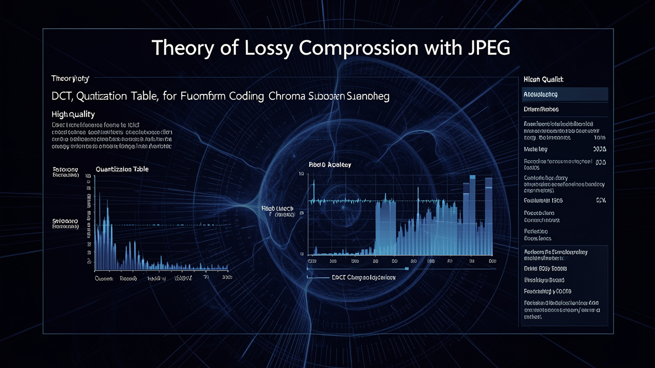
This is the step where the data is truly lost. Quantization is the process of mapping a large set of values to a smaller set. In JPEG, this is done by dividing each F(u,v) coefficient by a corresponding value from a quantization table. The result is then rounded to the nearest integer.
The quantization table is the key to controlling compression level and quality. JPEG provides two standard tables: one for luminance (Y) and one for chrominance (Cb/Cr). These tables are designed based on the human visual system’s sensitivity to different spatial frequencies. The human eye is most sensitive to low-frequency noise and least sensitive to high-frequency noise. Therefore, the quantization values in the table increase as you move from the top-left (low frequency) to the bottom-right (high frequency).
Example Luminance Quantization Table (Q_Y):
 16  11  10  16  24  40  51  61
 12  12  14  19  26  58  60  55
 14  13  16  24  40  57  69  56
 14  17  22  29  51  87  80  62
 18  22  37  56  68 109 103  77
 24  35  55  64  81 104 113  92
 49  64  78  87 103 121 120 101
 72  92  95  98 112 100 103  99
Notice how the values in the top-left are small (16, 11, 10). A small divisor means less quantization, preserving the important low-frequency data. The values in the bottom-right are large (101, 99, 103). A large divisor means more quantization, which will likely round the small high-frequency coefficients to zero.
The Quantization Process:
For each F(u,v) coefficient from our DCT output, we compute:
Quantized_Value(u,v) = round( F(u,v) / Q(u,v) )
Let’s apply this to our example DCT output. Using the first coefficient F(0,0) = 300 and Q(0,0) = 16:
Quantized_Value(0,0) = round(300 / 16) = round(18.75) = 19
For F(0,1) = -5 and Q(0,1) = 11:
Quantized_Value(0,1) = round(-5 / 11) = round(-0.4545) = 0
For F(1,0) = -6 and Q(1,0) = 12:
Quantized_Value(1,0) = round(-6 / 12) = round(-0.5) = -1 (or 0 depending on the rounding convention)
For all other F(u,v) coefficients which were 0:
Quantized_Value = round(0 / Q(u,v)) = 0
The result of quantization is a matrix that looks like this:
Quantized Coefficients:
  19   0   0   0   0   0   0   0
   0   0   0   0   0   0   0   0
   0   0   0   0   0   0   0   0
   0   0   0   0   0   0   0   0
   0   0   0   0   0   0   0   0
   0   0   0   0   0   0   0   0
   0   0   0   0   0   0   0   0
   0   0   0   0   0   0   0   0
We have reduced a complex block of 64 pixel values to just a single value (19) and a few zeros. This is the essence of JPEG’s lossy power. The “loss” is the information that was in the discarded high-frequency coefficients.
Quality Factor (Q-Factor): This is the single most important parameter for a user. A Q-factor of 100 means you are using a quantization table scaled down by a factor (e.g., Q/10), which means very little quantization, resulting in a near-lossless image but a large file. A Q-factor of 1 means you are scaling the quantization table up (e.g., Q * 50), ruthlessly discarding almost all high-frequency data, resulting in a tiny, severely degraded file. The standard JPEG tables are for a Q-factor of 50. The visual difference between a Q-factor of 85 and 95 is almost imperceptible, but the file size difference can be a factor of 2-3. This is the “sweet spot” for web use.
Step 6: The Phantom, The Runner, and The Huffman Tree
After quantization, we are left with a sparse matrix of numbers, mostly zeros. Our final task is to encode this matrix into a stream of bits as compactly as possible. This is done in a two-stage process: a spatial reordering called “zig-zag scan,” followed by a lossless entropy coding scheme, usually Huffman coding.
The Zig-Zag Scan:
The quantized coefficients are not read row-by-row or column-by-column. Instead, they are read in a diagonal zig-zag pattern starting from the top-left corner (the DC coefficient) and ending at the bottom-right corner. The purpose is to group the non-zero coefficients (which are concentrated in the top-left) together, followed by a long run of zeros.
Our quantized matrix [19, 0, 0, 0, ...] will be scanned as a sequence: [19, 0, 0, 0, 0, 0, 0, 0, 0, ...] (a long string of zeros).
Run-Length Encoding (RLE) and Huffman Coding:
This sequence is then coded using a hybrid scheme. The process is different for the DC coefficient (the first one) and the AC coefficients (the rest).
DC Coefficient: The DC coefficient is encoded differentially. Instead of storing the absolute value (19), we store the difference between the current block’s DC coefficient and the previous block’s DC coefficient. This is because neighboring 8x8 blocks tend to have similar average brightness, so the differences are very small and can be encoded with fewer bits. This difference is then Huffman-coded.
AC Coefficients: The remaining 63 coefficients are encoded using a form of Run-Length Encoding. The idea is to represent the sequence of coefficients as a series of (run, level) pairs.
- Run is the number of zeros that appear before a non-zero coefficient.
- Level is the value of the non-zero coefficient.
For our sequence [19, 0, 0, 0, ...], we have:
- First, we handle the DC coefficient (19).
- Then, we are at the start of the AC coefficients. The first non-zero coefficient is… none. They are all zero. In this case, we use a special symbol called End-of-Block (EOB), which means “all remaining coefficients are zero.”
So the entire AC sequence for our block is just the EOB symbol.
If our quantized matrix had two non-zero coefficients, e.g., [19, -3, 0, 0, 0, 5, 0, 0, ...], it would be encoded as:
- Encode DC coefficient (19).
- AC Run 1:
(0, -3)- zero zeros before-3. - AC Run 2:
(3, 5)- three zeros before5. - EOB symbol.
Huffman Coding:
Now we have a sequence of symbols: the differentially coded DC coefficient and the (run, level) pairs for the AC coefficients. Huffman coding is a variable-length coding technique that assigns shorter bitcodes to more frequently occurring symbols and longer bitcodes to less frequent symbols.
JPEG specifies default Huffman tables that are derived from the statistical distribution of coefficients in “typical” photographic images. A symbol like (0, 1) (a single zero before a coefficient of 1 or -1) is very common and will be assigned a short code (e.g., “001”). An obscure symbol like (15, 127) (15 zeros before a coefficient of 127 or -127) is extremely rare and will be assigned a very long code (e.g., “1111111110001”). The EOB symbol is also very common and gets a short code.
This final step can achieve a compression ratio of 2:1 to 3:1 on the already-quantized coefficients. When combined with chroma subsampling, the total compression ratio can easily reach 20:1 or more, with little to no visible degradation.
The Decoding Process: Reconstructing the Image
Decoding is the reverse of the encoding process, but it is not lossless. There is a critical step called dequantization. To reconstruct the image, we take the quantized coefficients (e.g., 19) and multiply them by the same quantization table value used during encoding.
Reconstructed_F(0,0) = 19 * 16 = 304
Notice that the original F(0,0) was 300, but we now have 304. This is the quantization error. This small error will be spread across the entire 8x8 block by the Inverse Discrete Cosine Transform (IDCT). The IDCT uses the same cosine basis functions to convert the frequency coefficients back into pixel values. Because we lost the high-frequency coefficients (they became zero), the reconstructed block will be a low-pass filtered, slightly smoothed version of the original.
Advanced Topics and JPEG Variations
Progressive JPEG: Instead of loading an image line by line from top to bottom (baseline JPEG), progressive JPEG loads the image in a series of scans. The first scan contains the low-frequency DCT coefficients for all blocks, giving a blurry, full-sized preview. Subsequent scans add higher-frequency coefficients, refining the image detail. This is excellent for slow internet connections, as users see a recognizable image very quickly.
JPEG 2000: The JPEG committee created a successor standard in 2000. It uses a fundamentally different transform called the Discrete Wavelet Transform (DWT) instead of the 8x8 block-based DCT. This eliminates the blocking artifact entirely and provides superior compression ratios, especially at high compression levels. It also supports lossless compression and a more sophisticated region-of-interest coding. Despite its technical superiority, JPEG 2000 never achieved widespread consumer adoption, partly due to patent issues and the massive existing ecosystem for standard JPEG.
Lossless JPEG: JPEG does define a lossless mode, using a completely different algorithm based on predictive coding instead of the DCT. However, it offers much lower compression ratios than lossy JPEG and is rarely used.
Metadata and EXIF: A JPEG file is not just compressed image data. It’s a container format that can store metadata. The Exchangeable Image File Format (EXIF) is a standard for storing camera settings (camera model, lens, aperture, shutter speed, ISO, date/time, GPS location) directly within the JPEG file. This metadata is read by almost all image viewing software.
Conclusion: The Elegant Ruthlessness
JPEG is a masterpiece of engineering that has quietly powered the visual internet for over three decades. Its genius lies not in a single brilliant idea, but in the perfect orchestration of multiple, carefully chosen techniques. It ruthlessly exploits the known weaknesses of the human visual system, from our poor color acuity (chroma subsampling) to our insensitivity to fine detail (DCT and quantization). It then uses elegant mathematics (DCT) and clever coding (Huffman) to package the remaining information with remarkable efficiency.
The result is an algorithm that, with a simple slider adjustment (quality factor), can tune itself from a near-perfect, lossless-looking archive to a highly compressed, “good enough” thumbnail. It is a perfect example of the principle that to communicate effectively, you must first understand what your audience does not need to see. In a world drowning in data, JPEG’s lesson in elegant ruthlessness is more relevant than ever. It is the invisible art of throwing data away, and it is, without a doubt, one of the most important algorithms of the digital age.