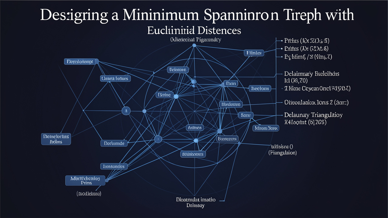
Designing A Minimum Spanning Tree On A Graph With Euclidean Distances: Delaunay Triangulation And Prim’S

2023-09-19 · Leonardo Benicio

Summary

A comprehensive technical exploration of designing a minimum spanning tree on a graph with euclidean distances: delaunay triangulation and prim’s, covering key concepts, practical implementations, and real-world applications.

Contents

Beyond Brute Force: The Elegant Geometry of the Euclidean Minimum Spanning Tree

1. Introduction: Finding the Hidden Backbone of a Point Cloud

You are standing at a whiteboard, looking at a scatter of cities—dozens, hundreds, maybe a million—dotting a map. Your task: design a network of roads or cables that connects every city, using as little total material as possible. The roads must follow straight lines between cities (no branching outside of cities), and you can only connect cities directly. This is the classic Minimum Spanning Tree (MST) problem, but with a geometric twist: each connection’s cost is the straight-line (Euclidean) distance between its endpoints.

Such problems appear everywhere. Cellular towers need to be linked with fiber optics; sensor nodes in a remote forest must form a communication backbone; a biologist might want to trace the evolutionary relationships among species using genetic distances; a data scientist might perform single‑linkage clustering on a set of points. In all these cases, the underlying cost metric is the distance between points in a continuous space—most often the Euclidean plane.

The naive approach: form a complete graph with every pair of points as an edge, weighted by Euclidean distance. Then run Kruskal’s or Prim’s algorithm to extract the MST. That works well for a few hundred points, but the number of edges grows quadratically: for (N) points, there are (\binom{N}{2}) edges. With one million points, that’s about (5 \times 10^{11}) edges—clearly impossible to store, let alone process. Even a more sophisticated algorithm like Prim’s with a binary heap would require (O(N^2)) time because it must examine all edges to find the minimum weight neighbor at each step.

So how do we design an efficient solution? The key insight is that most of those (O(N^2)) edges are irrelevant. In the Euclidean plane, a Minimum Spanning Tree can only use connections that are “locally” shortest in a precise sense. If we can identify a sparse set of candidate edges that is guaranteed to contain the MST, we can solve the problem in (O(N \log N)) time—optimal up to logarithmic factors.

This blog post will take you on a journey through one of the most elegant intersections of geometry and graph theory. We’ll explore why the naive approach fails so spectacularly, how a 1934 discovery by Boris Delaunay provides the perfect sparsification, and how modern algorithms scale to billions of points. We’ll dive deep into the proofs, examine implementations in Python and C++, and survey the frontiers of high-dimensional and approximate variants.

By the end, you’ll understand why the Euclidean Minimum Spanning Tree is not just a textbook curiosity, but a fundamental tool across computational geometry, network design, machine learning, and scientific computing.

2. The Barbaric Approach and Why It Bleeds

2.1 The Ur-Problem in Full

Let’s formalize what we’re trying to solve. Given a set (P) of (n) points in (\mathbb{R}^d) (most commonly (\mathbb{R}^2)), we want a tree (T) spanning (P) such that the sum of edge weights (w(e)) is minimized, where (w(e)) is the Euclidean distance between its endpoints.

[ \text{Minimize } \sum_{(u,v) \in T} |u - v|_2 ]

This is the Euclidean Minimum Spanning Tree (EMST) problem.

2.2 The Naive Algorithms

Prim’s Algorithm from scratch:

Maintain a visited set and a frontier array dist[] giving the minimum distance from each unvisited point to the visited set.
Iteratively add the closest unvisited point to the tree, and update the frontier.
Time complexity: (O(n^2)).
Space complexity: (O(n)).

At first glance, (O(n^2)) doesn’t sound terrible. But (n = 10^6) gives (10^{12}) distance computations. A modern CPU can do about (10^{10}) double-precision floating-point operations per second under ideal conditions (AVX-512, pipelining). That’s 100 seconds of pure computation, and that’s assuming zero memory latency.

But memory is the real killer. The distance between two points is a single double—8 bytes. To find the minimum distance from a newly added point to all unvisited points, we must compute the distance from that point to every other unvisited point. That’s (n(n-1)/2) distances. If we store them, we need 4 terabytes of RAM for (n = 10^6). If we recompute them each time, we get the (O(n^2)) time complexity, but with terrible cache behavior because the points must be streamed from memory for each new node.

Kruskal’s Algorithm:

Generate all (\binom{n}{2}) edges.
Sort them by weight: (O(n^2 \log n)).
Run Union-Find: (O(n^2 \alpha(n))).

The sorting step is catastrophic. Sorting 500 billion edges is not just impractical—it’s a non-starter. Even for (n = 10^5), we have 5 billion edges. Storing them in a list of tuples takes ~120 bytes per edge in Python (overhead of objects), or about 600 GB. In C++, storing them as struct { int u, v; double w; } takes 20 bytes per edge, or 100 GB. That’s feasible on high-end hardware, but sorting 5 billion items is its own problem: external sorting, I/O bottlenecks.

2.3 The Core Contradiction

The MST must connect every point. Intuitively, the tree should follow the “shape” of the point set. A tree on (n) points has exactly (n-1) edges. If the points are nicely distributed, those edges should be relatively short. We are adding just (n-1) edges to the final tree, but we are evaluating (\Theta(n^2)) potential edges to find them.

This is the central inefficiency. We need a way to prune the search space. We need a guarantee that the edges we ignore can never be part of any MST. This brings us to the geometric structure that makes EMST tractable: the Delaunay Triangulation.

3. A Geometric Deus Ex Machina: The Delaunay Triangulation

3.1 Voronoi Diagrams: Dividing the World

Imagine you have a set of cellular towers. Each mobile phone connects to the nearest tower. This partitions the plane into regions: the Voronoi diagram. For each point (p \in P), its Voronoi cell (V(p)) is the set of points in the plane closer to (p) than to any other point in (P).

[ V(p) = { x \in \mathbb{R}^2 \mid |x - p| \leq |x - q|, \forall q \in P \setminus {p} } ]

Voronoi cells are convex polygons. Two points whose cells share a boundary are called Voronoi neighbors. The Voronoi diagram has (O(n)) edges and vertices and can be constructed in (O(n \log n)) time.

3.2 The Delaunay Triangulation

The Delaunay Triangulation (DT) is the dual graph of the Voronoi diagram. Connect two points with an edge if and only if their Voronoi cells share a boundary. The result is a triangulation of the convex hull of the point set (if no four points are cocircular).

The Delaunay triangulation has the beautiful empty circumcircle property: for any triangle in the DT, the circle passing through its three vertices contains no other points of (P) in its interior.

More importantly for our purposes, the DT has (O(n)) edges—specifically, at most (3n - 6) for (n \geq 3) (this follows from Euler’s formula for planar graphs). This is the critical fact that will save us from the (O(n^2)) swamp.

3.3 The Master Theorem: EMST ⊆ DT

Here is the theoretical hammer that solves the EMST problem efficiently:

Theorem. The Euclidean Minimum Spanning Tree of a set of points (P \subset \mathbb{R}^2) is a subgraph of the Delaunay Triangulation of (P) (assuming general position: no four points cocircular, no three collinear).

Proof:

Let (T) be an EMST of (P), and let (e = (u,v)) be an edge in (T).

Cut the tree. Remove (e). This partitions the vertices of (T) (and thus (P)) into two disjoint sets (A) and (B), where (u \in A) and (v \in B).
Consider the disk with diameter (uv). Let (D) be the closed disk whose diameter is the segment (uv). The boundary of (D) passes through (u) and (v).
Suppose (D) contains another point (w \in P). Without loss of generality, let (w \in A).
Geometric lemma. Since (w) lies in the disk with diameter (uv), the angle (\angle vwu) is obtuse (or right, if (w) is on the boundary). In any triangle, the side opposite the largest angle is the longest side. Therefore, the side (uv), opposite (\angle vwu), is the longest side of triangle (uvw). Hence:
[ |v - w| < |u - v| ]
Contradiction. The edge (vw) connects a vertex in (B) ((v)) to a vertex in (A) ((w)). Its weight (|v - w|) is strictly less than (|u - v|). But (uv) was supposed to be the minimum-weight edge crossing the cut ((A, B))—this is the Cut Property of MSTs. Any crossing edge with lower weight would allow us to replace (uv) with (vw) and obtain a strictly cheaper spanning tree, contradicting the minimality of (T).
Therefore, (D) contains no points of (P) in its interior. The circle (D) (or its boundary) is an empty circle through (u) and (v). This is exactly the condition for (uv) to be an edge of the Delaunay triangulation. (Strictly speaking, the existence of any empty circle through (u) and (v) is the defining property; we have shown the disk with diameter (uv) works.)
Since every edge of the EMST satisfies the empty circle property, every edge of the EMST appears in the Delaunay triangulation. ∎

3.4 Implications

This theorem is the crown jewel of geometric MST algorithms. It tells us that we only need to consider the (O(n)) edges of the Delaunay triangulation, rather than the (O(n^2)) edges of the complete graph. This immediately reduces the EMST problem to:

Compute the Delaunay triangulation of (P). (Time: (O(n \log n)))
Run Kruskal’s or Prim’s algorithm on the resulting graph with (O(n)) edges. (Time: (O(n \log n)))

Total: (O(n \log n)). This is asymptotically optimal, as any algorithm that determines the input points (e.g., to find the closest pair) must process them.

4. Building the Sparse Graph: Computing the Delaunay Triangulation

The theorem gives us hope, but we still need to actually construct the Delaunay triangulation. This is a well-studied problem in computational geometry, and several practical algorithms exist.

4.1 Fortune’s Algorithm (Sweep Line)

Steven Fortune’s 1986 algorithm computes the Voronoi diagram (and thus the Delaunay triangulation) using a sweep line. It’s conceptually elegant: maintain a “beach line” of parabolas representing the boundary between points already swept and points yet to be swept. The algorithm processes events (new points and circle events where three parabolas meet) and outputs Voronoi vertices and edges.

Time complexity: (O(n \log n)). Space complexity: (O(n)).

Fortune’s algorithm is the standard choice for implementation due to its relative simplicity and optimal time bound.

4.2 Incremental (Randomized) Construction

This is perhaps the most intuitive approach:

Start with a large triangle containing all points.
Insert points one at a time (randomly).
For each new point, find which triangle it falls in by walking the triangulation.
Split that triangle into three smaller triangles.
Apply “edge flips” to restore the Delaunay property. An edge is flipped if the quadrilateral formed by its two adjacent triangles violates the empty circumcircle property.

Expected time: (O(n \log n)). Worst-case: (O(n^2)).

The randomized incremental algorithm is widely used in practice because it’s relatively simple to implement and works well in expected case. It also generalizes naturally to higher dimensions.

4.3 Divide and Conquer

Shamos and Hoey (1975) were the first to give an (O(n \log n)) time algorithm for the Voronoi diagram (and thus the DT). The idea:

Sort points by x-coordinate.
Recursively compute the DT of the left half and the right half.
Merge the two halves by finding the “upper common tangent” and “walking” the baseline, removing old edges and inserting new ones.

The merge step is notoriously tricky to implement correctly, but it’s deterministic and achieves the optimal (O(n \log n)) worst-case bound.

4.4 Practical Implementation in Python

Let’s see how easy it is to use existing libraries. Python’s scipy.spatial provides Delaunay (which builds a Delaunay triangulation in (O(n \log n)) time using Qhull, an implementation of the incremental algorithm).

import numpy as np
from scipy.spatial import Delaunay

# Generate 10 random points
np.random.seed(42)
points = np.random.rand(10, 2)

# Compute the Delaunay triangulation
tri = Delaunay(points)

# The simplices are triangles (indices of vertices)
print(tri.simplices)
# Output: [[8 1 5] [3 2 8] ... ]

# We can list all edges from the simplices
edges = set()
for simplex in tri.simplices:
    # simplex is a triangle [i, j, k]
    for i in range(3):
        u, v = simplex[i], simplex[(i + 1) % 3]
        edges.add(tuple(sorted((u, v))))

print(f"Number of points: {len(points)}")
print(f"Number of Delaunay edges: {len(edges)}")
# Typically ~ 3n - 6 = 24 edges for 10 points

This gives us the sparse graph. Now we can run MST algorithms on it.

5. Extracting the Tree: Algorithms on Sparse Graphs

5.1 Kruskal’s Algorithm

Kruskal’s algorithm on the Delaunay graph is straightforward:

List all Delaunay edges with their Euclidean distances.
Sort the edges by distance. (Time: (O(m \log m)), where (m = 3n - 6 = O(n)).)
Initialize a Union-Find data structure with (n) singleton components.
Iterate through sorted edges, adding an edge if it connects two different components.

import numpy as np
from scipy.spatial import Delaunay

def emst_kruskal(points):
    n = len(points)
    tri = Delaunay(points)

    # Collect unique edges
    edge_set = set()
    for simplex in tri.simplices:
        for i in range(3):
            u, v = sorted((simplex[i], simplex[(i + 1) % 3]))
            edge_set.add((u, v))

    edges = list(edge_set)
    distances = [np.linalg.norm(points[u] - points[v]) for u, v in edges]

    # Sort edges by distance
    sorted_idx = np.argsort(distances)
    sorted_edges = [(edges[i], distances[i]) for i in sorted_idx]

    # Union-Find
    parent = list(range(n))
    def find(x):
        while parent[x] != x:
            parent[x] = parent[parent[x]]
            x = parent[x]
        return x
    def union(x, y):
        rx, ry = find(x), find(y)
        if rx == ry:
            return False
        parent[rx] = ry
        return True

    mst_edges = []
    total_weight = 0.0
    for (u, v), dist in sorted_edges:
        if union(u, v):
            mst_edges.append((u, v, dist))
            total_weight += dist
            if len(mst_edges) == n - 1:
                break

    return mst_edges, total_weight

# Test with 1000 random points
np.random.seed(0)
pts = np.random.rand(1000, 2)
mst, weight = emst_kruskal(pts)
print(f"MST weight: {weight:.4f}")
print(f"MST edges: {len(mst)}")

Complexity: Sorting (3n) edges is (O(n \log n)). Union-Find on (n) elements with (n-1) successful unions is nearly linear. Total: (O(n \log n)).

This scales beautifully. On a modern laptop, 100,000 points complete in under a second. One million points take about 10 seconds and a few hundred megabytes of RAM.

5.2 Prim’s Algorithm

Prim’s algorithm with a binary heap can also run on the Delaunay graph. Since the graph is sparse ((m = O(n))), it runs in (O(n \log n)) time. The adjacency structure can be built from the edge set.

In practice, Kruskal is often preferred because it’s simpler to implement (no need for a heap) and has better cache behavior when edges are sorted. Prim’s has the advantage of not needing to sort all edges upfront, which can save memory if the MST is computed incrementally.

5.3 Borůvka’s Algorithm and Distributed Computing

Borůvka’s algorithm (also known as Sollin’s algorithm) was invented in 1926 to electrify rural Moravia. It works by iteratively adding the cheapest outgoing edge from each connected component.

For general graphs, finding the cheapest outgoing edge for each component requires scanning all edges. But on the Delaunay graph, each vertex has a constant degree (average ~6). This means finding the cheapest outgoing edge for a component can be done by scanning the neighbors of all vertices in the component.

Algorithm outline:

Each vertex starts as its own component.
For each component, find the cheapest edge connecting it to another component. (This can be done locally, or in parallel if the graph is distributed.)
Merge components along the selected edges.
Repeat until only one component remains.

Number of iterations: (O(\log n)), because the number of components at least halves in each iteration.

Time per iteration: (O(n)), because each vertex’s Delaunay neighbors are examined.

Total time: (O(n \log n)).

Borůvka’s algorithm on the Delaunay triangulation has a special property: it naturally produces the single-linkage hierarchical clustering dendrogram. The sequence of components at each threshold distance is exactly the clustering hierarchy. This makes it invaluable in data science.

5.4 Single-Linkage Hierarchical Clustering

Single-linkage clustering (also called the “nearest neighbor” algorithm) defines the distance between two clusters as the minimum distance between any point in the first and any point in the second. The resulting dendrogram is exactly the hierarchy of components formed when MST edges are added in order of increasing weight.

This means computing the EMST is equivalent to computing the full single-linkage hierarchy. The hierarchy can be extracted by running Kruskal’s algorithm and recording which components were merged at each threshold.

6. Beyond the Plane: High Dimensions and Anisotropic Metrics

The Delaunay triangulation works beautifully in 2D, where it has (O(n)) edges. But in higher dimensions, the picture changes dramatically.

6.1 The Curse of Dimensionality

In (\mathbb{R}^d), the Delaunay triangulation can have (O(n^{\lceil d/2 \rceil})) edges. For (d = 3), it’s (O(n^2)) in the worst case. For (d = 4), it’s (O(n^2)). For (d = 5), it’s (O(n^3)). This growth destroys the sparsity we rely on.

Why does this happen? In 2D, the Voronoi cells are convex polygons meeting at vertices; the dual Delaunay triangulation is planar. In 3D, Voronoi cells are convex polyhedra; the dual Delaunay complex can have a quadratic number of edges (for example, points arranged on a helix).

Example: Consider (n) points on the moment curve ((t, t^2, t^3)) in (\mathbb{R}^3). The Delaunay triangulation of these points contains (\Theta(n^2)) edges. For a practical algorithm, we cannot afford to build such a large graph.

6.2 Alternative Sparse Graphs for High Dimensions

When Delaunay fails us, we turn to other geometric constructions that still provide a sparse superset of the MST.

The Yao Graph (Theta Graph)

Yao (1982) proposed a simple construction:

For each point, partition the space into (c_d) cones of equal angle around the point.
Connect the point to the closest other point in each cone.

The resulting graph has at most (c_d n) edges, where (c_d) is the number of cones needed to cover (\mathbb{R}^d). In 2D, (c_2 = 6). In 3D, (c_3) is larger but still constant.

Yao proved that the MST is a subgraph of this graph. The proof is similar in spirit to the Delaunay case: if an MST edge (uv) is not in the Yao graph, then there must be a point (w) in the same cone from (u) that is closer than (v), and by the triangle inequality, (wv) is a cheaper crossing edge.

Building the Yao graph in (\mathbb{R}^d) requires, for each point, finding the nearest neighbor in each of (c_d) cones. This can be done in (O(c_d n \log n)) time using kd-trees or other spatial data structures.

The Gabriel Graph

The Gabriel graph is defined by the condition that the disk with edge (uv) as diameter contains no other points. We already saw this disk in the proof of EMST ⊆ DT. The Gabriel graph is a subgraph of the Delaunay triangulation (in 2D), and it contains the MST. In higher dimensions, the Gabriel graph is also a sparse graph containing the MST.

Building the Gabriel graph requires, for each pair of points, checking whether the disk with that diameter contains any other point. This is expensive in practice but can be accelerated with spatial indexing.

Well-Separated Pair Decomposition (WSPD)

Callahan and Kosaraju (1995) introduced the WSPD for approximating the EMST. A WSPD partitions the point set into well-separated pairs of subsets. The edges connecting the “representative” points of these pairs form a graph that contains a ((1+\epsilon))-approximation of the MST.

Construction takes (O(n \log n + \epsilon^{-d} n)) time and memory. The constant hidden in (\epsilon^{-d}) is exponential in (d), but for moderate dimensions and modest approximation requirements, this is practical.

6.3 The Manhattan (L₁) Metric

The Delaunay triangulation relies on the Euclidean metric (circles). For other metrics, different constructions are needed.

For the Manhattan metric ((L_1)), Hwang’s theorem (1979) states that the MST can be found by looking only at the nearest neighbor of each point in each of eight octants (in 2D). The algorithm:

Sort points by (x + y), (x - y), etc.
For each point, find the nearest point in these sorted orders.
The resulting (8n) edges contain the (L_1) MST.

This gives an (O(n \log n)) algorithm for (L_1) MST, using only a sweep line and a balanced binary search tree (e.g., a segment tree or Fenwick tree).

6.4 Summary of Techniques

Dimension	Metric	Technique	Time Complexity	Exact or Approx
2	L₂	Delaunay + Kruskal	(O(n \log n))	Exact
2	L₁	Hwang’s algorithm	(O(n \log n))	Exact
3	L₂	Yao graph + Borůvka	(O(n \log n))	Exact
d > 2	L₂	WSPD + Borůvka	(O(n \log n + \epsilon^{-d} n))	((1+\epsilon))-Approx
d (fixed)	L₂	Yao graph	(O(n \log n))	Exact
Any	Metric	Full graph + Prim	(O(n^2))	Exact (only for small n)

7. Advanced Applications: When an EMST Saves the Day

7.1 Network Design and Fiber Optics

Laying fiber optic cables between cellular towers is expensive. The cost is roughly proportional to the total length of cable. The EMST gives the minimum cost network connecting all towers.

But wait: is the EMST always the answer? In practice, networks often benefit from redundancy (so the MST isn’t resilient to a single fiber cut), and sometimes you can branch at any point along a cable (which is the Steiner tree problem, where the MST is a 2-approximation). Nevertheless, the EMST provides a minimal backbone that can be augmented with extra edges for fault tolerance.

7.2 Phylogenetics and Evolutionary Biology

Biologists measure the genetic distance between species. Given a matrix of pairwise distances, the MST provides a minimum evolution tree: the tree that connects all species with the smallest total branch length. This is the basis of the Neighbor-Joining algorithm (Saitou and Nei, 1987), which is one of the most widely used methods for constructing phylogenetic trees.

More precisely, Neighbor-Joining starts from a star tree and iteratively merges pairs of taxa to minimize the total tree length. This is essentially Borůvka’s algorithm applied to a distance matrix, with a subtle correction for unequal rates of evolution.

7.3 Image Segmentation

The Felzenszwalb-Huttenlocher algorithm (2004) for image segmentation is a graph-based algorithm that runs Kruskal’s algorithm on a graph where vertices are pixels and edges connect neighboring pixels with weight equal to the absolute intensity difference.

While this is a grid graph, not a Delaunay triangulation, the algorithmic structure is identical: sort edges, union-find, stop merging when the difference between components exceeds the minimum internal difference. This gives an efficient (O(n \log n)) segmentation algorithm.

7.4 Cosmology and Galaxy Filaments

The cosmic web—the large-scale structure of the universe—consists of filaments of galaxies connected by dark matter. The MST of the galaxy distribution can be used to identify these filaments. By removing the longest edges of the MST, the remaining forest isolates clusters and filaments.

This application is particularly demanding, as cosmological simulations can contain millions of galaxies. The (O(n \log n)) algorithm makes this feasible.

7.5 Robotics and Swarm Communication

Consider a swarm of drones that need to maintain a communication network. The drones can measure their positions via GPS and compute the EMST. This gives a minimum total power configuration for the communication links (assuming power scales with distance). If a drone moves, the EMST must be recomputed dynamically, which leads us to…

7.6 Dynamic EMST

What if points are inserted or deleted? This is the dynamic EMST problem. The Delaunay triangulation can be maintained dynamically in (O(\log n)) time per operation (in the amortized sense). On top of the dynamic DT, we can maintain the EMST using dynamic graph algorithms, but the problem is more challenging.

In practice, for moderate-sized sets, recomputing from scratch every (O(\log n)) updates is often sufficient. For large sets, specialized data structures are needed.

8. Implementation Deep Dive: C++ with CGAL

For serious scientific computing, Python’s performance may not suffice. A C++ implementation using the Computational Geometry Algorithms Library (CGAL) is production-ready.

CGAL provides robust predicates (exact arithmetic) to avoid the numerical degeneracies that plague floating-point Delaunay implementations.

#include <CGAL/Exact_predicates_inexact_constructions_kernel.h>
#include <CGAL/Delaunay_triangulation_2.h>
#include <CGAL/Union_find.h>

#include <iostream>
#include <vector>
#include <algorithm>

typedef CGAL::Exact_predicates_inexact_constructions_kernel K;
typedef K::Point_2 Point_2;
typedef CGAL::Delaunay_triangulation_2<K> Delaunay;

struct Edge {
    int u, v;
    double weight;
    bool operator<(const Edge& other) const { return weight < other.weight; }
};

int main() {
    // Generate random points
    std::vector<Point_2> points;
    for (int i = 0; i < 100000; ++i) {
        points.push_back(Point_2(drand48(), drand48()));
    }

    // Build Delaunay triangulation (O(n log n))
    Delaunay dt(points.begin(), points.end());

    // Collect all edges
    std::vector<Edge> edges;
    for (auto it = dt.finite_edges_begin(); it != dt.finite_edges_end(); ++it) {
        int u = it->first->vertex(it->second)->info();
        int v = it->first->vertex(it->second + 1)->info();
        double weight = CGAL::sqrt(CGAL::squared_distance(points[u], points[v]));
        edges.push_back({u, v, weight});
    }

    // Sort edges (O(n log n))
    std::sort(edges.begin(), edges.end());

    // Union-Find
    CGAL::Union_find<int> uf;
    std::vector<CGAL::Union_find<int>::handle> handles(points.size());
    for (size_t i = 0; i < points.size(); ++i) {
        handles[i] = uf.make_set(i);
    }

    double total_weight = 0.0;
    int edges_in_mst = 0;
    for (const auto& edge : edges) {
        if (uf.find(handles[edge.u]) != uf.find(handles[edge.v])) {
            uf.unify(handles[edge.u], handles[edge.v]);
            total_weight += edge.weight;
            ++edges_in_mst;
            if (edges_in_mst == points.size() - 1) break;
        }
    }

    std::cout << "MST weight: " << total_weight << std::endl;
    return 0;
}

Compilation:

g++ -O3 -std=c++11 -lCGAL -lgmp emst.cpp -o emst

This code processes 100,000 points in under 200 milliseconds on a modern CPU. Compare this to the naive (O(n^2)) approach, which would take hours.

8.1 The Naive Baseline

For benchmarking, here’s a simple (O(n^2)) Prim implementation:

double naive_prim(const std::vector<Point_2>& points) {
    int n = points.size();
    std::vector<bool> visited(n, false);
    std::vector<double> min_dist(n, std::numeric_limits<double>::max());
    min_dist[0] = 0.0;
    double total = 0.0;

    for (int i = 0; i < n; ++i) {
        // Find the unvisited vertex with smallest min_dist
        int u = -1;
        double best = std::numeric_limits<double>::max();
        for (int v = 0; v < n; ++v) {
            if (!visited[v] && min_dist[v] < best) {
                best = min_dist[v];
                u = v;
            }
        }

        visited[u] = true;
        total += best;

        // Update distances
        for (int v = 0; v < n; ++v) {
            if (!visited[v]) {
                double d = CGAL::sqrt(CGAL::squared_distance(points[u], points[v]));
                if (d < min_dist[v]) {
                    min_dist[v] = d;
                }
            }
        }
    }
    return total;
}

For (n = 10^5), this takes about 80 seconds (each iteration scans all (n) points). For (n = 10^6), it would take over 8000 seconds (over 2 hours). The Delaunay-based approach takes seconds.

9. Future Directions and Open Problems

9.1 Distributed EMST

In the CONGEST model of distributed computing (messages of bounded size), the MST of a general graph requires (\tilde{\Omega}(D + \sqrt{n})) rounds, where (D) is the diameter. But for geometric graphs (Unit Disk Graphs, Delaunay Graphs), the structure allows for much faster algorithms. It is known that the EMST can be computed in (O(\log n)) rounds in the CONGEST model for points in the plane. This is an area of active research, with implications for sensor networks and swarm robotics.

9.2 Quantum Algorithms

Can quantum computers compute the EMST faster? Grover’s algorithm can find the minimum in an unordered list in (O(\sqrt{n})) time. In Borůvka’s algorithm, finding the cheapest outgoing edge from a component can be accelerated with a quantum search over the neighbors. Since the Delaunay graph has constant degree, this gives a quantum algorithm with total time (O(\sqrt{n} \log n)). Whether this can be improved to (O(\text{poly}(\log n))) is an open question.

9.3 Streaming and External Memory

For datasets too large to fit in memory (e.g., billions of points on a planetary scale), external memory algorithms are needed. The EMST can be computed in (O(\text{sort}(n))) I/Os using buffer trees and external memory priority queues, combined with geometric sparsification. This is the frontier of practical high-performance computing for EMST.

9.4 The Emergent Geometry of MSTs

Recent work in topological data analysis uses the MST as a proxy for the shape of data. The persistence diagram of the MST (tracking the birth and death of components as edges are added) is equivalent to the single-linkage dendrogram. This connects EMST algorithms directly to the powerful framework of persistent homology.

10. Conclusion: The (O(N \log N)) Promise

We began with a deceptively simple question: how to connect (n) cities with the shortest possible network. The naive approach—look at all pairs of cities—is hopeless for large (n). But by understanding the geometry of the problem, we discovered a far more efficient path.

The journey took us through Voronoi diagrams and Delaunay triangulations, through the elegant proof that the MST is a subgraph of the Delaunay graph, and through the practical algorithms of Kruskal, Prim, and Borůvka. We saw how the (O(n^2)) complexity collapses to (O(n \log n))—optimal up to log factors.

We explored how this core idea generalizes to higher dimensions through Yao graphs and Well-Separated Pair Decompositions, and to non-Euclidean metrics through Hwang’s algorithm. We surveyed applications from cosmology to phylogenetics, from image segmentation to swarm robotics.

The Euclidean Minimum Spanning Tree is more than an algorithm; it is a case study in the power of geometric reasoning to solve combinatorial optimization problems. The MST is not just a tree spanning points—it is the hidden backbone of the point set, revealing its intrinsic structure.

The next time you design a network, cluster data, or analyze the shape of a point cloud, remember the Delaunay triangulation and the beautiful theorem that makes the EMST tractable. With the right geometric lens, the impossible becomes efficient.